Project 2 - Rankine cycle Simulator

AIM: To study Rankine cycle and create a Rankine cycle simulator

OBJECTIVE:

• To simulate a Rankine Cycle using MATLAB.
• Extracting steam and water properties from XSteam data(IAPWS - 97 standard)
• Calculating all the state points of the cycle based on user inputs.
• Plotting the T vs s and H vs s plot for the given input.

Rankine Cycle:

The Rankine cycle is an idealized thermodynamic cycle describing the process by which certain heat engines, such as steam turbines or reciprocating steam engines, allow mechanical work to be extracted from a fluid as it moves between a heat source and heat sink.

Heat energy is supplied to the system via a boiler where the working fluid (typically water) is converted to a high pressure gaseous state (steam) in order to turn a turbine. After passing over the turbine the fluid is allowed to condense back into a liquid state as waste heat energy is rejected before being returned to boiler, completing the cycle. Friction losses throughout the system are often neglected for the purpose of simplifying calculations as such losses are usually much less significant than thermodynamic losses, especially in larger systems.

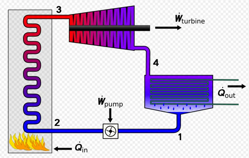
1. Pump, 2. Boiler, 3. Turbine, 4. Condenser.

In this project the idealised Rankine cycle is simulated by neglecting the losses. Rankine cycle is derived out of Carnot cycle. Its power depends upon the temperature difference between the heat source and a cold source. The more the difference in heat the more will be the efficiency of the mechanical power generation. Since ideal cycles are only in theory, Efficiency of Rankine cycle is limited by high heat of vaporization of the working fluid, friction losses etc

The fluid used in a Rankine cycle is water due to its favourable properties, such as its non-toxic and unreactive, Abundant and low cost, good thermodynamic properties. The efficiency of the cycle is higher as the pump consumes only 1-3% of the turbine output power.

Process and working:

The Rankine cycle follows four steps:

1. Process 1-2: Isentropic Expansion in the turbine
2. Process 2-3: Constant pressure heat rejection in condenser
3. Process 3-4: Isentropic compression in the pump
4. Process 4-1: Constant pressure heat addition in the boiler

Working of a Rankine Cycle:

1. In process 1-2, The dry saturated vapour expands through a turbine and generates power. This decreases the temperature and pressure of the vapour.
2. In process 2-3, Due to decrease in temperature the vapour gets condensed at low pressure. The condensation occurs because of a cooling water. In a well-designed condenser, the pressure of vapour is well below atmospheric pressure, approaching the saturation pressure of the operating fluid at the cooling water temperature.

• In process 3-4, The pressure of the condensate is raised in the feed pump. Because of the low specific volume of liquids, the pump work is relatively small and often neglected in thermodynamic calculations.

1. Process 4-1, High pressure liquid enters the boiler from the feed pump, and is heated to saturation temperature. Further addition of energy causes evaporation of liquid until it is fully converted to saturated steam or superheated.

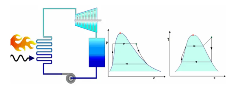
Thermodynamic Equations and formulae:

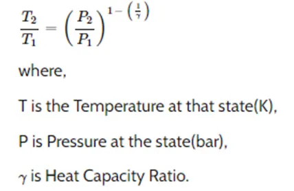
For Isentropic expansion:

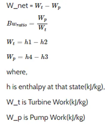
For Net work(W net) and back work ratio(Bw ratio):

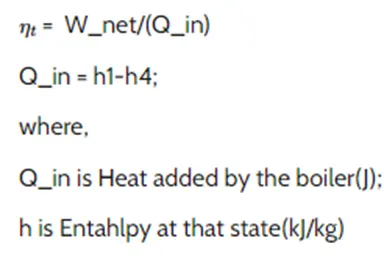
For Thermal Efficiency:

MATLAB PROGRAM:

%% Rankine cycle simulator

% Objective of this program to simulate rankine cycle 
% plot T-s and H-s diagram using data from Xsteam data 
% Water and steam properties according to IAPWS IF-97

close all
clear all
clc

disp('                  RANKINE CYCLE                   ');
disp('1-2 is Iscentropic Expansion in the Turbine');
disp('2-3 is constant pressure heat rejecttion by the condensor');
disp('3-4 is Iscentropic Expansion in the pump');
disp('4-1 is constant pressure heat addition to the boiler');

%Inputs:
disp('                  INPUTS                  ');
P1 = input('Enter the pressure at the turbine inlet(bar):');
T1 = input('Enter the temperature at the turbine inlet(degree C):');
P2 = input('Enter the pressure at the condenser(bar):');

% Using XSteam functions, the enthalpy and entropy at various points can be
% calculated:

% Calculating enthalpy(h) and entropy(s) at point1:
h1 = XSteam('h_pT',P1,T1);
s1 = XSteam('s_pT',P1,T1);

%calculating pressure(P), enthalpy(h) and entropy(s) at point2:

% Since Iscentropic Expansion:
s2 = s1;
% For Iscentropic Expansion:
%wkt (T2/T1) = (P2/P1)^(1-(1/g))
g = 1.4;
power = 1 - (1/g);

% Hence (T2/T1) = (P2/P1)^power:
T2 = T1*((P2/P1)^power);
h2 = XSteam('h_pT',P2,T2);

% Calculating pressure(P),enthalpy(h) and entropy(s) at point 3:
% Since constant pressure heat removal:
P3 = P2;
T3 = T2;
h3 = XSteam('hL_T',T3);
s3 = XSteam('sL_T',T3);

% Calculating pressure(P),enthalpy(h) and entropy(s) at point 4:
% Since Iscentropic Compression:
s4 = s3;

% Since Constant pressure process:
P4 = P1;

T4 = XSteam('T_ps',P4,s4);
h4 = XSteam('h_pT',P4,T4);
h41 = XSteam('hL_p',P4);
s41 = XSteam('sL_p',P4);
h42 = XSteam('hV_p',P4);
s42 = XSteam('sV_p',P4);
T41 = XSteam('T_hs',h41,s41);
T42 = XSteam('T_hs',h42,s42);

% calculating the Entropy and Enthalpy at the saturation curve:
Temp = linspace(0,500,600);

for i = 1:length(Temp)

sv(i) = XSteam('sV_T',Temp(i));
sl(i) = XSteam('sL_T',Temp(i));
 
hv(i) = XSteam('hV_T',Temp(i));
hl(i) = XSteam('hL_T',Temp(i));

end

% Calculating the net work output (W_net):

W_t = h1-h2;
W_p = h4-h3;
W_net = W_t-W_p;

% Calculating the back work ratio:
Bw_ratio = W_p/W_t;

% Calculating the thermal efficiency:
Q_in = h1-h4;
eff_thermal = (W_net/Q_in)*100;

% Caluculating Specific Steam consumption:
% wkt 1J = 3600kg/s
SSC = 3600/W_net;

% Displayinh the result in the command window:
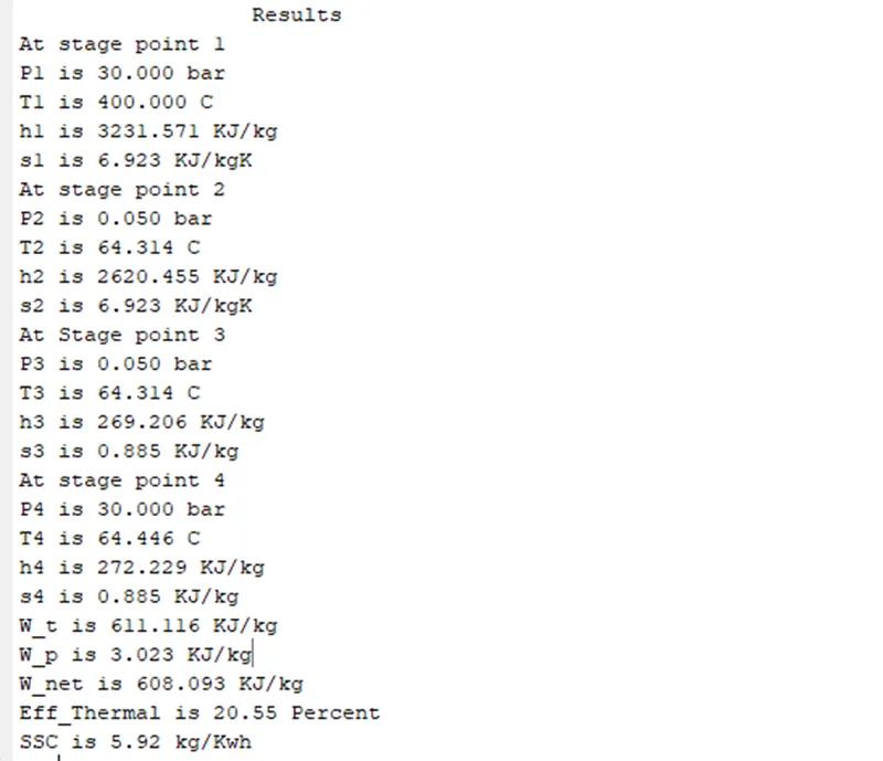
disp('                  Results                 ');
P1 = P1;
T1 = T1;
P2 = P2;
disp('At stage point 1');
n1 = sprintf('P1 is %.3f bar',P1);
disp(n1);
n2 = sprintf('T1 is %.3f C',T1);
disp(n2);
n3 = sprintf('h1 is %.3f KJ/kg',h1);
disp(n3);
n4 = sprintf('s1 is %.3f KJ/kgK',s1);
disp(n4);
disp('At stage point 2');
n11 = sprintf('P2 is %.3f bar',P2);
disp(n11);
n21 = sprintf('T2 is %.3f C',T2);
disp(n21);
n31 = sprintf('h2 is %.3f KJ/kg',h2);
disp(n31);
n41 = sprintf('s2 is %.3f KJ/kgK',s2);
disp(n41);
disp('At Stage point 3');
n12 = sprintf('P3 is %.3f bar',P3);
disp(n12);
n22 = sprintf('T3 is %.3f C',T3);
disp(n22);
n32 = sprintf('h3 is %.3f KJ/kg',h3);
disp(n32);
n42 = sprintf('s3 is %.3f KJ/kg',s3);
disp(n42);
disp('At stage point 4');
n13 = sprintf('P4 is %.3f bar',P4);
disp(n13);
n23 = sprintf('T4 is %.3f C',T4);
disp(n23);
n33 = sprintf('h4 is %.3f KJ/kg',h4);
disp(n33);
n43 = sprintf('s4 is %.3f KJ/kg',s4);
disp(n43);
n14 = sprintf('W_t is %.3f KJ/kg',W_t);
disp(n14);
n15 = sprintf('W_p is %.3f KJ/kg',W_p);
disp(n15);
n16 = sprintf('W_net is %.3f KJ/kg',W_net);
disp(n16);
n17 = sprintf('Eff_Thermal is %.2f Percent',eff_thermal);
disp(n17);
n18 = sprintf('SSC is %.2f kg/Kwh',SSC);
disp(n18);

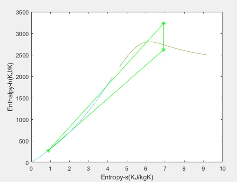
figure(1)
plot([s1 s2],[h1 h2],[s2 s3],[h2 h3],[s3 s4],[h3 h4],[s4 s1],[h4 h1],'marker','*','color','g')
hold on
plot(sv,hv)
plot(sl,hl)
xlabel('Entropy-s(KJ/kgK)');
ylabel('Enthalpy-h(KJ/K)');

OUTPUT:

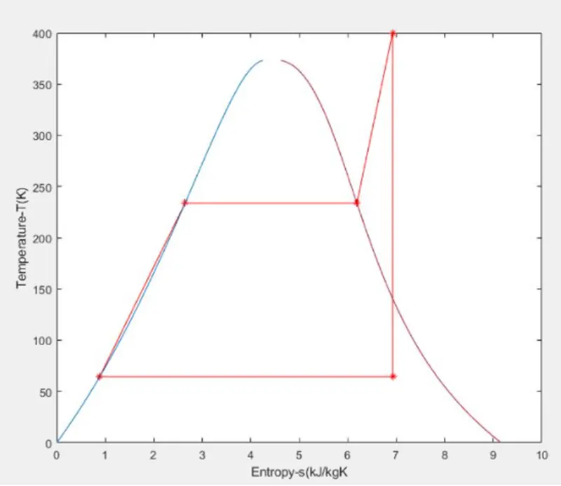
T-S diagram:

H-S Diagram:

Results and Conclusion:

The performance of the Heat engine was calculated and the following observations were made:

1. Net Work = 608.093KJ/kg
   2. Thermal Efficiency = 20.55 %
   3. Back Work Ratio = 0.4%