Week 4.1 - Genetic Algorithm

Optimisation

Optimisation is the method used to find the maximum or minimum of function subjected to various constraints and input parameters. The objective of optimisation on maximiising or minimising the function totally depend upon the application of the function.

For eg: maximising the fuel efficiency of engine, finding the fastest route between two locations, minimising the risk in financial investments etc. can all be represented as optimisation problems in real life.

A flow chart of how optimisation methods work is shown below

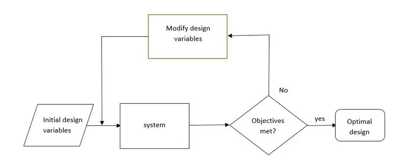
Every optimisation methods involve intial guessing of variables, and then check for either maximum or minimum. On acheiving a favourable feedback, the random inputs once initially guessed are then rechanged or reprogrammed to a newer set of variables to achieve a even better result than the previous execution. Thus the process continuoues further on until any pre-set criteria is met.

Hence optimisation is preffered for finding better optimal designs or for obtaining any faster design criteria .

Genetic algorithm

One of the optimisation methods provided in the matlab is the genetic algorithm solver, which incorporates the idea of genetic algorithm to find a optimised design from a random population.

In GA from a pool of solution, each solution undergo recombinations or mutations to produce children. The so solutions produced are then calculated for the fitness value, which indicates the best possible solution in the solution pool. Further these children still undergo recombinations, mutations to obtain a newer generation of solution that posses much better fitness value than the previous ones.

Here in genetic algorithm, from the random population, the components are made to undergo 3 processes that are vital to optimise the problem

• Selection operator

In selection,from the pool of poulation each individual is calculated for its fitness value. The individual having scored the highest fitness value is then selected as the best possible solution or output and is selected as the 'parent'. The ones scoring least fitness value are then discarded. The cycle can continue to produce more 'child' from each selected 'parents', leading to better optimal solution from the random population. For selection various methods are used such as tournament method,roulette wheel method,proportionate selction, rank selection etc. These involves the calculation of fitness value and predicting the overall probability of each solution involved to be selected as the 'parent'.

• Mutation

During mutation, the components can undergo changes by itself to score more fitness value. The one's mutated better, i.e has higher fitness value is then passed on to the next generation. These random mutations prevent the solution from stalling on to a single solution even though best solution from selection method alone is obtained.

• Cross-over

During recombinations, the child produced from parent of previous generation can attain characteristics of parent, by restructing itself to produce more fitness value.This cross-over helps to find even better solution for an optimisation problem

A diagramatic representation of how these wor is shown below:

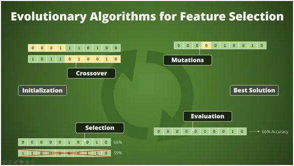
Genetic algorithm for optimisation problem

Genetic algorithm problems are mainly used for solving problems involving non-linear function or non-differentiable form functions that are needed to be optimised. In traditional methods, that involve calculating the gradient, after starting at a random point, it is possible that the solution may get stuck at a local minima/maxima. Hence, the solution wont converge to find the global minima or maxima. In many real world problems, the functions are non smooth and involve mulitle peaks of local minima/maxima that may not be better represented in differentiable form with a global minima/maxima. Such functions are optimised with the help of genetic algorithm.

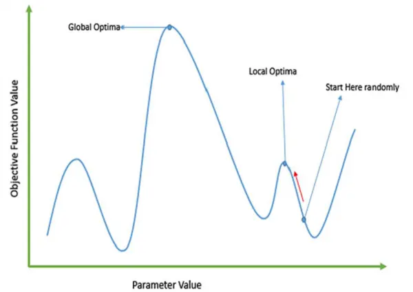
In matlab genetic algorithm is used to find the global minima of the function. Hence to find the global maxima, we simply find the minima of its negative function.

Synatx of ga

• For a given function say f(x) it is important that while passing the function, the no. of variables (nvar) involved must be passed on.
• Also while the function assumes random variables for each population, it is important that the search space such as upper or lower limit of input parameters must be given. This is important as many practical problems involve limitation upto which they can vary the parameter. So the optimal solution must be obtained in this range. Hence upper and lower bounds are given. for eg, the lower bound is passed as lb=[0 0] and upper bound as ub=[5 5]
• If the function is constrained by another linear equation and linear unequal equation , then they must also be passed on to the ga syntax , to let the function know that the solutions obtained must also comply to the constrained equation.
• for eg: consider the constrained equations,`x+y>=3` and `y==3+x`, then at first greater than inequality constraints are converted to less then inequality constraint, and is made into matrix form to pass on to the ga syntax. Hence the equation is rewritten as `-x-y<=-3` and `-x+y==3`. The coeffiecients of variables and the RHS are seperately passed to the synatx of ga in matrix form. i.e`A=[-1 -1]`and `b=-3`, for linear equal constraints, `Aeq=[-1 1]`and `beq=3`
• if non-linear constraints are used then the keyword 'nonlcon' is used to specify that constraint, the non-linear constraint will be a pre-defined function with the non-linear equation in it.
• If we have constriants in integer value, then the keyword 'intcon' is used. This denotes that upon reaching the fitness value a predefined integer, the function stop optimising.
• The diagonising of the ga is done by using the keyword 'options'. Using the options, we can plot the minimum value obtained during each iteration and the best fitness value for that population using 'gaplotbestf' and we can also visualise what made the function optimise using 'gaplotstopping'. Also the population size considered for each evaluation can be restricted or increased by using the keyword 'PopulationSize`. By default 'ga'considers 50 random variables as its default size`.
• also if there are none of the factors involved for optimising the function, then '[]' is used to indicate that function is not constrainted to above conditions at their respective entry points.

The syntax of ga can be given as [x,fval,exitflag,output]=ga(fun_name,nvar,A,b,Aeq,beq,nonlcon,intcon,options)

Here x is the vector that gives the position where global minima is obtained, 'fval' gives the value obtained at this position, 'exitflag' denotes what condition made the condition stopping from further optimising which is related to constraints discussed above, and 'output' gives the details of population , such as no. of interations, the no. of generations it took to meet the objective etc

Stopping criteria of ga optimisation

The no. of iterations can either be manually set or stops when the stopping criteria is met.

• MaxGenerations- The algorithm stops when the number of generations reaches maximum Generations

• MaxTime - The algorithm stops after running for an amount of time in seconds equal to MaxTime

• FitnessLimit - The algorithm stops when the value of the fitness function for the best point in the current population is less than or equal to FitnessLimit.

• MaxStallGenerations - The algorithm stops when the average relative change in the fitness function value over MaxStallGenerations is less than FunctionTolerance

• MaxStallTime - The algorithm stops if there is no improvement in the objective function during an interval of time in seconds equal to MaxStallTime

• FunctionTolerance- The algorithm runs until the average relative change in the fitness function value over MaxStallGenerations is less than FunctionTolerance.

• ConstraintTolerance - The ConstraintTolerance is not used as stopping criterion. It is used to determine the feasibility with respect to nonlinear constraints.

Optimising the stalagmite function

The stalagmite function is given as

`f(x,y)=f(1,x).f(2,x).f(1,y).f(2,y)`

`f(1,x)=[sin(5.1pix+0.5)]^6`

`f(2,x)=e[-4ln(2).(x-0.0667)^2/0.64]`

`f(1,y)=[sin(5.1piy+0.5)]^6`

`f(2,y)=e[-4ln(2).(y-0.0667)^2/0.64]`

At first the stalagmite function is coded as a function. while coding since ga only minimises a function, we have to put negative to find the maximum of the given function

i.e max(f(x,y))=min(-f(x,y))

The stalagmite function is then plotted

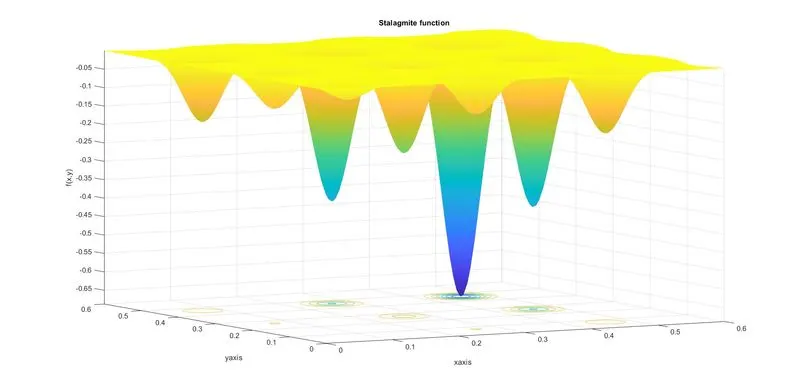
Study1

Now we are going to optimise the given function. For this in study 1 we plot the stalagmite function, but the optimisation isnt subjected to any constraints. Due to this the results we obtain are plotted inaccordance with the random values of x and y the ga algorithm randomly taken. This is of no practical significance as constraining and finding the optimum solution within the constrain is the practical application view of ga. The plot obtained in study 1 is

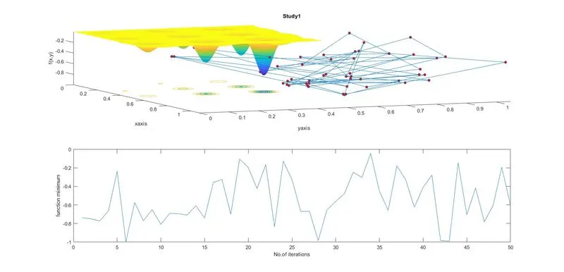
From the figure it is clear that ga optimised the function by taking random variables which are out of any bounds or constraints, hence was unable to converge to find a global minimum.

Study2

For the study2, the lower and upper bounds are passed to the function. Hence while initialising random population, the value ga assumes may lie in between the lower and upper bounds specified as [0 0] and [0.6 0.6]. We also use tic and toc command to calculate the time taken by solver to iterate through 50 iterations. SInce the function bounds are given, the chances of converging the optimisation to a global minimum is the highest. The graph is obtained as below.

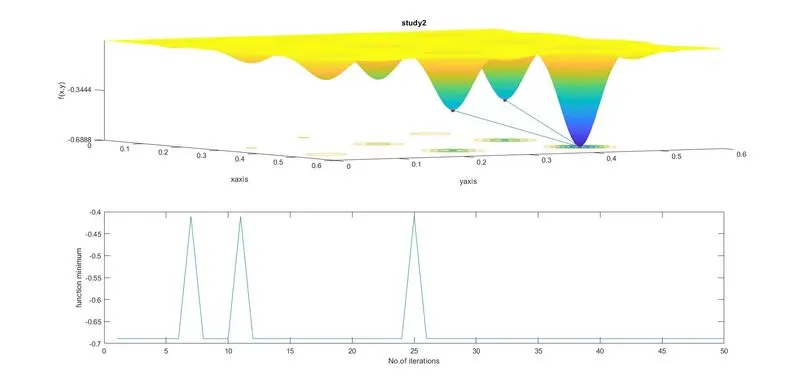
Now it is evidant from comparing study 1 and study 2 that optimisation has given a better result when the function is executed in specified bounds. Still the global minimum is not obtained. For this study 3 is conducted

Study3

By default, ga assumes 50 random variables for each generation. Here for study3, the populationsize is increased. This is attained by setting the population size to higher value by using the keyword 'PopulationSize' in options. Also the best plot function graph is plotted as well as the plot stopping condition graph is plotted as well.

At first the population size is increased to 60, and the results are plotted

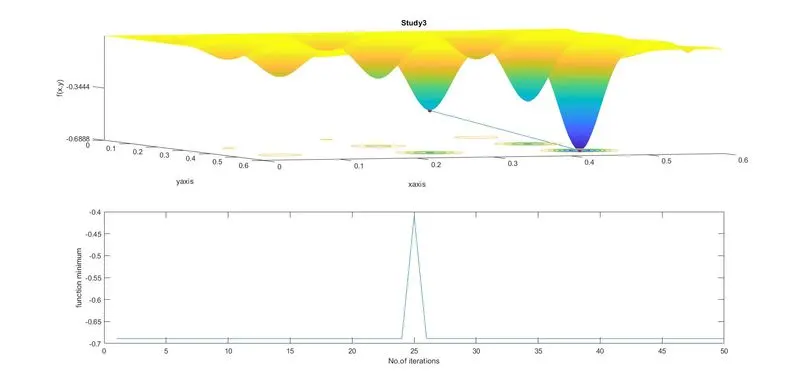
Here its obsereved that global minimum is still not achieved. Hence the population size is further increased.

the study time observed was

This is considerably higher than one that was done with less number of population.

Now the population is increased to 150, the graph obtained is

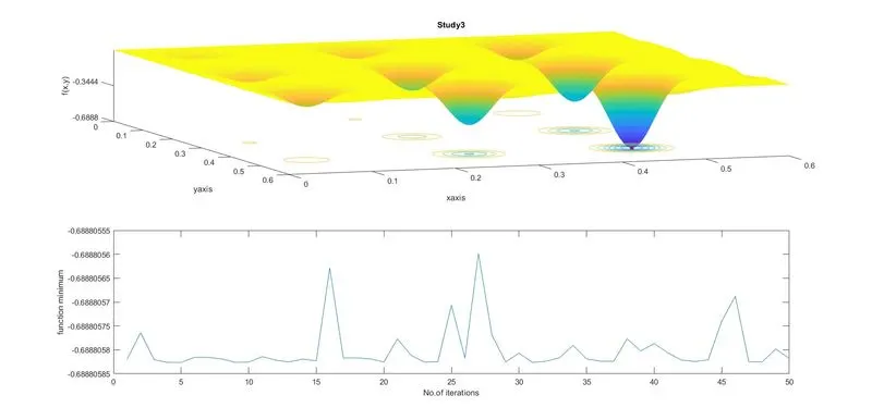
Hence by increasing the population of the pool, the global minimum of the function is obtained. The results are

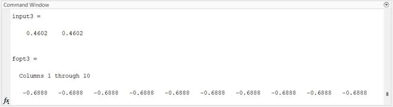
The x and y cordinates for the minumum value -0.688 is (0.4602,0.4602).

The bestplotf and plotstopping graphs are obtained , the following figure represent the results ga obtained while iterating for the 50th time

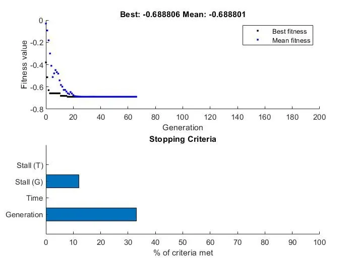
The stall(G) represent that after how many generations, the f(x,y) stall onto the optimum solution, Generation represent, the no. of generations, the random variables had to undergo all the selection, mutation and cross-over process to obtain the optimum solution.

Here the minimum of the function -f(x,y) is determined which is the maximum location of stalagmite function f(x,y).

REFERENCE

• Find minimum of function using genetic algorithm - MATLAB ga - MathWorks 한국
• How the Genetic Algorithm Works - MATLAB & Simulink - MathWorks India
• Genetic Algorithms - Introduction (tutorialspoint.com)
• GA Selection operators (iitg.ac.in)

clear all
close all
clc

% Creating x and y values for plotting the stalagmite function
x=linspace(0,0.6,150);
y=linspace(0,0.6,150);

% Creating a 2-D matrix
[xx,yy]=meshgrid(x,y);

% Evaluating the stalgamite function
for i=1:length(xx)
    for j=1:length(yy)
        input_vector(1)=xx(i,j);
        input_vector(2)=yy(i,j);
        f(i,j)=stalagmite(input_vector);
    end 
end

surfc(xx,yy,f)
xlabel('xaxis');
ylabel('yaxis');
zlabel('f(x,y)');
shading interp
title('Stalagmite function');

num_case=50;   % num_cases is the no.of iterations since it denotes, the no. of times x and
%                y values are passed on for stalagmite function

toc
for i=1:num_case;
    [input1,fopt1(i)]=ga(@stalagmite,2);
        xopt1(i)=input1(1);
        yopt1(i)=input1(2);
end
study1_time=toc

% Plotting the stalagmite function and optimising the function without
% providing any bounds or constraints
% 
% Study 1

figure(1)
subplot(2,1,1)
hold on
% Plotting the stalagmite function

surfc(xx,yy,f)
xlabel('xaxis')
ylabel('yaxis')
zlabel('f(x,y)')

title('Study1')
shading interp

% Plotting the minimum values obtained for each iteration

plot3(xopt1,yopt1,fopt1,'marker','o','markersize',5,'markerfacecolor','r'); 

subplot(2,1,2)
plot(fopt1)
xlabel('No.of iterations');
ylabel('function minimum');

% Plotting the stalagmite function and optimising the function by
% providing upper and lower bounds with 0 < x-cordinate <0.6 and 
% 0 < y-cordinate < 0.6
% [] denote the function is not constrianed to linear ineqaulities or
% linear equalities
% 
% study2

tic
for i=1:num_case;
[input2,fopt2(i)]=ga(@stalagmite,2,[],[],[],[],[0 0],[0.6 0.6]);
xopt2(i)=input2(1);
yopt2(i)=input2(2);
end
study2_time=toc

figure(2)
subplot(2,1,1)
hold on
surfc(xx,yy,f)
xlabel('xaxis')
ylabel('yaxis')
zlabel('f(x,y)')
title('study2')
shading interp
plot3(xopt2,yopt2,fopt2,'marker','o','markersize',5,'markerfacecolor','r')
subplot(2,1,2)
plot(fopt2)
xlabel('No.of iterations');
ylabel('function minimum');


% Study 3

% The population sizen is increased to find the global minimum of the
% function
% the plot stopping f value graph and best fvalue graph is plotted

options=optimoptions('ga','PlotFcn',{@gaplotbestf,@gaplotstopping},'populationsize',150);
tic
for i=1:num_case;
[input3,fopt3(i),output]=ga(@stalagmite,2,[],[],[],[],[0;0],[0.6;0.6],[],[],options)
xopt3(i)=input3(1);
yopt3(i)=input3(2);
end
study3time=toc

figure(3)
subplot(2,1,1)
hold on
surfc(xx,yy,f)
xlabel('xaxis')
ylabel('yaxis')
zlabel('f(x,y)')
title('Study3')
shading interp
plot3(xopt3,yopt3,fopt3,'marker','o','markersize',5,'markerfacecolor','r')
subplot(2,1,2)
plot(fopt3)
xlabel('No.of iterations');
ylabel('function minimum');




% the function stalagmite is coded as

% function[m]=stalagmite(input_vector)
% 
% a=input_vector(1);
% b=input_vector(2);
% f1=(sin(5.1.*pi.*a+0.5)).^6;
% f2=(sin(5.1.*pi.*b+0.5)).^6;
% 
% 
% f3=exp(-4.*log(2).*(((a-0.667).^2)./0.64));
% f4=exp(-4.*log(2).*(((b-0.667).^2)./0.64));
% 
% m=-(f1.*f2.*f3.*f4); 
% 
% end
%