Week 4.1 - Genetic Algorithm
AIM
To write a Matlab program to optimize the stalagmite function to find the global maxima of that function
OBJECTIVE
- To write a code in MATLAB to optimise the stalagmite function and to find the global maxima of the function.
- To expalin the concept of genetic algorithm and to explain the syntax for ga in MATLAB.
THEORY OF GENETIC ALGORITHM
- Genetic algorithms are based on the ideas of natural selection and genetics.
- These are intelligent exploitation of random search provided with historical data to direct the search into the region of better performance in solution space.
- They are commonly used to generate high-quality solutions for optimization problems and search problems.
- Genetic algorithms simulate the process of natural selection which means those species who can adapt to changes in their environment are able to survive and reproduce and go to next generation.
- In simple words, they simulate “survival of the fittest” among individual of consecutive generation for solving a problem.
- Each generation consist of a population of individuals and each individual represents a point in search space and possible solution.
- Each individual is represented as a string of character.
- Genetic algorithms are based on an analogy with genetic structure and behavior of chromosomes of the population.
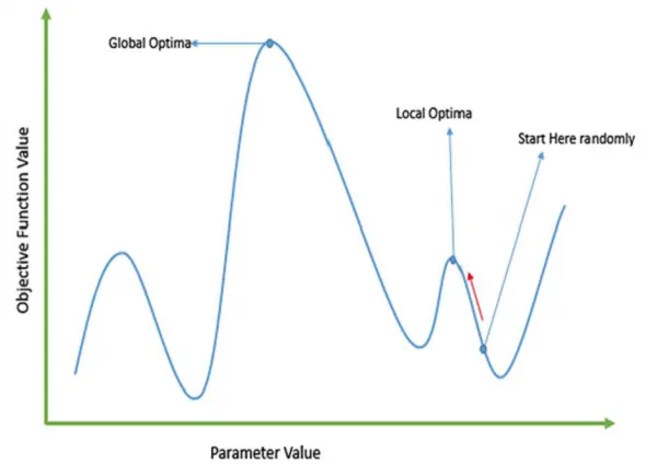
Initialization of Population (Coding)
The code generates its random population of defined size and from that population the code evaluates the fitness of the members of the population according to which it forms new population based on no. of iterations performed.
Fitness Function
It is that function which we have to optimize and its optimization is done with the help of number of generations which have been formed by the code accordance with the fitness value of each member generated, these fitness values are used for the reproduction of the children.
Selection
The idea of the selection phase is to select the fittest individuals and let them pass their genes to the next generation. The main goal of this phase is to find the region where the chances of getting the best solution are more.
Inspiration for this is from the survival of the fittest.
It should be a balance between exploration and exploitation of search space.
GA tries to move the genotype to higher fitness in the search space.
Too strong fitness selection bias can lead to sub-optimal solutions.
Too little fitness bias selection results in unfocused search.
Reproduction
Generation of offspring happen in 2 way:
Crossover
Mutation
A) Crossover
Crossover is the most significant stage in the genetic algorithm. During crossover, a random point is selected while mating a pair of parents to generate offspring.
There are 3 major types of crossover.
Single Point Crossover:
A point on both parents’ chromosomes is picked randomly, and designated a ‘crossover point’.
Two-Point Crossover: Two crossover points are picked randomly from the parent chromosomes.
Unifofm Crossover: In a uniform crossover, typically, each bit is chosen from either parent with equal probability.
B) Mutation
In a few new offspring formed, some of their genes can be subjected to a mutation with a low random probability. This indicates that some of the bits in the bit chromosome can be flipped. Mutation happens to take care of diversity among the population and stop premature convergence.
SYNTAX FOR GENETIC ALGORITHM
x = ga(fun, nvars,A,b,Aeq,beq,lb,ub)
x = ga(fun,nvars,A,b,Aeq,beq,lb,ub,nonlcon)
x = ga(fun,nvars,A,b,Aeq,beq,lb,ub,nonlcon,options)
x = ga(fun,nvars,A,b,[],[],lb,ub,nonlcon,IntCon)
x = ga(fun,nvars,A,b,[],[],lb,ub,nonlcon,IntCon,options)
x = ga(fun,nvars) finds a local unconstrained minimum, x, to the objective function, fun. nvars is the dimension (number of design variables) of fun.
x = ga(fun,nvars,A,b) finds a local minimum x to fun, subject to the linear inequalities A*x ≤ b. ga evaluates the matrix product A*x as if x is transposed (A*x').
x = ga(fun,nvars,A,b,Aeq,beq) finds a local minimum x to fun, subject to the linear equalities Aeq*x = beq and A*x ≤ b. (Set A=[] and b=[] if no linear inequalities exist.) ga evaluates the matrix product Aeq*x as if x is transposed (Aeq*x').
x = ga(fun,nvars,A,b,Aeq,beq,lb,ub) defines a set of lower and upper bounds on the design variables, x, so that a solution is found in the range lb ≤ x ≤ ub. (Set Aeq=[] and beq=[] if no linear equalities exist.)
x = ga(fun,nvars,A,b,Aeq,beq,lb,ub,nonlcon) subjects the minimization to the constraints defined in nonlcon. The function nonlcon accepts x and returns vectors C and Ceq, representing the nonlinear inequalities and equalities respectively. ga minimizes the fun such that C(x) ≤ 0 and Ceq(x) = 0. (Set lb=[] and ub=[] if no bounds exist.)
x = ga(fun,nvars,A,b,Aeq,beq,lb,ub,nonlcon,options) minimizes with the default optimization parameters replaced by values in options. (Set nonlcon=[] if no nonlinear constraints exist.) Create options using optimoptions.
x = ga(fun,nvars,A,b,[],[],lb,ub,nonlcon,IntCon) or x = ga(fun,nvars,A,b,[],[],lb,ub,nonlcon,IntCon,options) requires that the variables listed in IntCon take integer values.
x = ga(problem) finds the minimum for problem, a structure described in problem.
[x,fval] = ga(___), for any previous input arguments, also returns fval, the value of the fitness function at x.
[x,fval,exitflag,output] = ga(___) also returns exitflag, an integer identifying the reason the algorithm terminated, and output, a structure that contains output from each generation and other information about the performance of the algorithm.
[x,fval,exitflag,output,population,scores] = ga(___) also returns a matrix population, whose rows are the final population, and a vector scores, the scores of the final population.
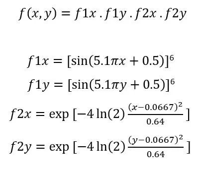
STALAGMITE FUNCTION EQUATION
PROGRAM FOR STALAGMITE FUNCTION
function [f] = stalagmite_function(input_vector)

x = input_vector(1);
y = input_vector(2);

f1x = (sin(5.1*pi*x + 0.5)).^6;
f1y = (sin(5.1*pi*y + 0.5)).^6;

f2x = exp(-4*log(2)*(((x-0.0667).^2)/0.64));
f2y = exp(-4*log(2)*(((y-0.0667).^2)/0.64));

f = -(f1x * f1y * f2x * f2y);

end
We start the function as the input vector for a functiom
let x be the input vector 1
and y be input vector 2
write the formula as the coding
finally we use the -ve sign so that the plot will be reversed as we have to find the maxima of the given function using ga.
PROGRAMMING AND DESCRICPTION
clear all
close all
clc

%Defining our Search Space

x = linspace(0,0.6,150);
y = linspace(0,0.6,150);

%Creating 2-D mesh

[xx,yy] = meshgrid(x,y);

%Evaluting the Stalagmite function

for i=1:length(xx)
    for j=1:length(yy)
        input_vector(1) = xx(i,j);
        input_vector(2) = yy(i,j);
        f(i,j) = stalagmite_function(input_vector);

    end
end
figure(1)
surfc(xx,yy,-f)
xlabel('x values')
ylabel('y values')
zlabel('z values')
shading interp
%[inputs , fval] = ga(@stalagmite_function,2)


num_cases = 80

tic

%Study 1  Statistical Behaviour

for i = 1:num_cases
    [input,fopt(i)] = ga(@stalagmite_function,2);
    xopt(i) = input(1);
    yopt(i) = input(2);
end

study1_time = toc


figure(2)
subplot(2,1,1)
hold on
surfc(x,y,f)
shading interp
plot3(xopt,yopt,fopt,'marker','o','MarkerSize',5,'MarkerfaceColor','r')
title('unbounded inputs')
subplot(2,1,2)
plot(fopt)

xlabel('iterations')
ylabel('function maximum')


tic

% Study 2  Statistical behaviour with upper and lower bounds

for i=1:num_cases
    [inputs, fopt(i)] = ga(@stalagmite_function,2,[],[],[],[],[0;0],[1;1]);
    xopt(i) = inputs(1);
    yopt(i) = inputs(2);
end

study2_time = toc


figure(3)
subplot(2,1,1)
hold on
surfc(x,y,f)
shading interp
plot3(xopt,yopt,fopt,'marker','o','MarkerSize',5,'MarkerfaceColor','r')
title('bounded inputs')
subplot(2,1,2)
plot(fopt)

xlabel('iterations')
ylabel('function maximum')

%Study 3 Increasing GA itreations

options = optimoptions('ga');
options = optimoptions(options,'PopulationSize',650);

tic


for i=1:num_cases
    [inputs, fopt(i)] = ga(@stalagmite_function,2,[],[],[],[],[0;0],[1;1],[],[],options);
    xopt(i) = inputs(1);
    yopt(i) = inputs(2);
end

study3_time = toc

figure(4)
subplot(2,1,1)
hold on
surfc(x,y,f)
shading interp
plot3(xopt,yopt,fopt,'marker','o','MarkerSize',5,'MarkerfaceColor','r')
title('bounded inputs with increased itretations')
subplot(2,1,2)
plot(fopt)


xlabel('iterations')
ylabel('function maximum')
Start the program using the commands
clear all
close all
clc
Firstly, creating the mesh from the two vectors x and y with values ranging from 0 to 0.6 with 150 vales between them using linspace command which will be acting as a search space to find the maxima of the function.
Creating the mesh of these two vectors using the ‘mesh’ command and defining the no. of iterations as num_cases to iterate the values of the optimum values of the function.
Now calculating the values of fitness function at each point of the mesh grid formed.
for loop is used for the complete length of x and y axis and the stalagmite function is called.
Now creating its surface through ‘surfc’ command which will also provide the contour of the generated surface.
Lable with x,y and z axis and Figure 1 is obtained.
Now the intial iteration is given as num_cases and here we taken 80 cases.
In First Study of STATISTICAL BEHAVIOUR the total time taken also calulated by starting tic command
The optimum value of fitness function at each iteration and calculating it using the above-mentioned first syntax
[input,fopt(i)] = ga(@stalagmite_function,2);
xopt(i) = input(1);
yopt(i) = input(2);
the time calculates ends with the command toc
Then plotting it into the surf command and also providing the optimum values of the function that how it is varying.
The plot obtained is further highlited using Marker Markersize and Markerfacecolor command.
Still the maximum values are varying from vast difference so it cannot be perfect
The time taken for the first study is 3.079 sec
In the second study STATISTICAL BEHAVIOUR WITH UPPER AND LOWER BOUNDS
Like the first study the same procedure is repeated with the addition of upper and lower limits
[inputs, fopt(i)] = ga(@stalagmite_function,2,[],[],[],[],[0;0],[1;1]);
For this the time taken is also calculated with tic toc command
The figure obtained is also highlited
The time taken for the study is 4.2026 sec
It is clearly seen from the above that after providing the boundary limits the variation in the optimum value of the function has reduced.
even with the upper and lower bounds the perfect maximum values is not comparable
So in the Third study WITH INCREASED ITERATIONS the values can be made to get clear
First the ga function is called with the syntax used to call the iterations and the number of populations.
here the population number is increased to 650
options = optimoptions('ga');
options = optimoptions(options,'PopulationSize',650);
Then the for loop is called for the syntax used for the calculation
[inputs, fopt(i)] = ga(@stalagmite_function,2,[],[],[],[],[0;0],[1;1],[],[],options);
Now the plot obtained is optimized to the extent.
The time taken for the code to run is also increased and taken 36.785 sec
ERRORS WHILE CODING
There are few errors occured while coding and the major error is the toolbox error,

I overcame the error by installing the Global Optimization Toolbox from the matlab which is essential in running the program
RESULT
Thus with the Genetic Algorithm a matlab code is generated for stalasmite function to fing the global maxima of the plot. It can be much more visualized that how the fitness is been calculated and best result is being displaced even with the increase in size of population
REFERENCES
What Is the Genetic Algorithm? - MATLAB & Simulink - MathWorks India