Project 2 - Rankine cycle Simulator

AIM:

 Create a Rankine Cycle simulator using MATLAB/Octave

OBJECTIVE:

Calculation of state points of any Rankine cycle Plotting of corresponding T-s and H-s curves of the cycle

THEORY

Vapour power cycle: The cycle in which vapour is used as a working substance is called a vapour power cycle.

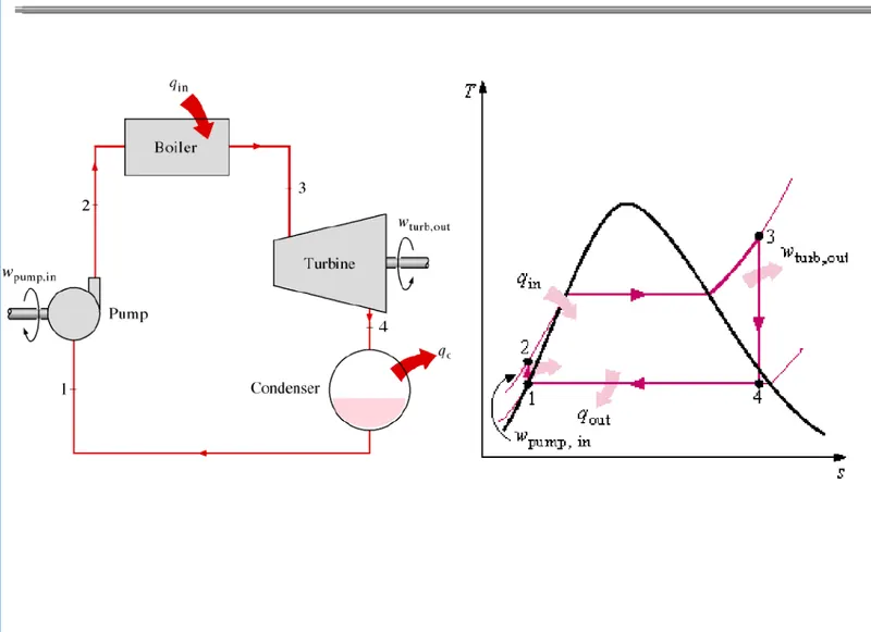
Rankine Cycle: Many impracticalities associated with the Carnot cycle can be eliminated by superheating the steam in the boiler and condensing it completely in the condenser. The resulting cycle is the Rankine cycle, which is ideal cycle for vapour power plants.

The ideal Rankine cycle does not involve any internal irreversibilities and consists of the following four processes:

 1-2: Isentropic expansion of steam in the turbine.

2-3: Isobaric heat rejection in the condenser.

3-4: Pumping of water from condenser into boiler. This process is isentropic.

4-1: Conversion of water into steam in boiler. This process is Isobaric heat addition.

 

Back Work Ratio: It is the ratio of pump work input to the work developed by the turbine.

Specific Fuel Consumption: It is the amount of steam required to procedure 1 kWh.

FORMULAS:

 For one kg of fluid flow

1. Heat supplied by fuel in the boiler

Qs = m(h1 − h2)

2. Work is done by the turbine

Wt = m(h1 − h2)η(turb)

3.Heat rejected by the steam in the condenser

Qr = m(h2 − h3)

4. Work input to the pump

Wp = mV 3(P4 − P3) ⋅ 10^2 /η(pump)

5. Net work is done

W = Wt – Wp

 6.The efficiency of the Rankine cycle

η = W/ Qs

7. Back work ratio = Wp/ Wt

8. Work ratio = W /Wt

9. Specific steam consumption rate SSC = 3600/ W

h1,h2,h3,h4 are the enthalpy at the state points 1,2,3,and 4 respectively.

PROGRAM:

Steam table data has been provided in Xsteam file.

Program for simulating Rankine cycle is as follows:

%Rankine Cycle Simulator
clear all
close all
clc

%Output Header
fprintf('%70s \n \n \n','Rankine Cycle Simulator');
fprintf('1-2 is Isentropic Expansion in the turbine \n');
fprintf('2-3 is Constant Pressure Heat Rejection by the Condensor \n');
fprintf('3-4 is Isentropic Compression in the Pump \n');
fprintf('4-1 is Constant Pressure Heat Addition by the Boiler \n \n');

% inputs
p1=input(' Enter the Pressure at turbine inlet (in bar):\n');
t1=input(' Enter the Temperature at turbine inlet (in degrees):\n');
p2=input(' Enter the pressure at Condensor inlet (in bar):\n');

% extracting specific heat values using function XSteam
cp1_l = XSteam('CpL_p',p1);
cp1_v = XSteam('CpV_p',p1);
cp2_l = XSteam('CpL_p',p2);
cp2_v = XSteam('CpV_p',p2);

%inputs to the turbine
s1 = XSteam('s_pT',p1,t1);
h1 = XSteam('h_pt',p1,t1);

% condensor inlet
s2=s1; %1-2 is an isentropic expansion process
sf2=XSteam('sL_p',p2);
sg2=XSteam('sV_p',p2);
hf2=XSteam('hL_p',p2);
hg2=XSteam('hV_p',p2);

% saturated temperature
Tsat_p1 = XSteam('Tsat_p',p1);
Tsat_p2 = XSteam('Tsat_p',p2);

%calculating dryness fraction 
if(s2<=sg2)
    x2 = ((s2 - sf2) / (sg2-sf2)); % Dryness Fraction at state point 2
else
    x2=1; 
end

if (x2<1)
    t2 = Tsat_p2;
else
    S2 = Sg_2+cp2_v*(log(T2/Tsat_p2))
    t2 = (Tsat_p2+273.15)*exp((s2-sg2)/cp2_v);
    t2 = t2 - 273.15;
end

if(x2<1)
    h2=hf2+(x2*(hg2-hf2));
else
    h2=XSteam('h_pT',p2,t2);
end

% condensor exit

p3=p2;
t3=XSteam('Tsat_p',p3);
s3=XSteam('sL_p',p3);
h3=XSteam('hL_p',p3);
v3=XSteam('vL_p',p3);
t2=t3;

% boiler inlet
p4=p1; % constant pressure heat addition
s4=s3; %isentropic compression in the pump
h4=XSteam('h_ps',p4,s4);
cp4=XSteam('Cp_ps',p4,s4);
cv4=XSteam('Cv_ps',p4,s4);
g4=(cp4/cv4);

% calculation for t4

%p4^(1-gamma)*t4^gamma=p3^(1-gamma)*t3^gamma;
t4=(t3*((p3/p4)^((1-g4)/g4)));

% calculations
% work done by the turbine
Wt=h1-h2;

% work done by the pump
Wp=h4-h3;

% net work done
W_net=Wt-Wp;

% heat added in the boiler
q_in=h1-h4;

% heat rejected in the condensor
q_out=h2-h3;

% Thermal efficiency
n=(W_net/q_in)*100;

%Back Work Ratio
bwr = Wp/Wt;

%Steam Rate
ssc = 3600/W_net;

%plotting the results

figure(1)
%plotting liquid and vapour curves
t=linspace(1,t1,1000);

for i=1:length(t)
    s_l(i)=XSteam('sL_T',t(i));
end

for i=1:length(t)
    s_v(i)=XSteam('sV_T',t(i));
end

 hold on
 plot(s_l,t,'linewidth',2,'linestyle','--','color','r')
 plot(s_v,t,'linewidth',2,'linestyle','--','color','r')
 grid on

 % plotting for the work done by the turbine(process 1-2)
plot([s1,s2],[t1,t2],'linewidth',2,'color','b')
hold on
title(' T-S Diagram of Ideal Rankine Cycle')
xlabel('Entropy(KJ/KgK)')
ylabel('Temperature(k)')

% Plotting for heat rejected in condensor (Process 2-3)
plot([s2,s3],[t2,t3],'linewidth',2,'color','b')
hold on
% Plotting for work done by the pump (Process 3-4)/
plot([s3,s4],[t3,t4],'linewidth',2,'color','b')
hold on

% Plotting for heat added by the boiler(Process 4-1)
tp = XSteam('TSat_p',p4);
sp = XSteam('sL_T',tp);
plot([s4,sp],[t4,tp],'lineWidth',2,'color','b')
hold on
tq = tp;
sq = XSteam('sV_T',tq);
plot([sp,sq],[tp,tq],'lineWidth',2,'color','b')
hold on
plot([sq,s1],[tq,t1],'lineWidth',2,'color','b')
hold on

%Indicate states with numbers
text(s1,t1,' 1');
text(s2,t2,' 2');
text(s3,t3,' 3');
text(s4,t4,' 4');

%Plot for enthalpy vs entropy
figure(2)
plot([s1,s2],[h1,h2],'lineWidth',2,'color','b')
grid on
title('H-S DIAGRAM')
xlabel('Entropy(KJ/kgK)')
ylabel('Enthalpy(KJ/kg)')
hold on
plot([s2,s3],[h2,h3],'lineWidth',2,'color','b')
hold on
plot([s3,s4],[h3,h4],'lineWidth',2,'color','b')
hold on
plot([s4,s1],[h4,h1],'lineWidth',2,'color','b')

%plot for liqiuid and vapour saturation curve
t = linspace(1,t1,1000);

for j = 1:length(t)
    h_l(j) = XSteam('hL_T',t(j));
end


for j = 1:length(t)
    h_v(j) = XSteam('hV_T',t(j));
end

plot(s_l,h_l,'lineWidth',2,'color','r')
hold on
plot(s_v,h_v,'lineWidth',2,'color','r')

%Indicate states with numbers
text(s1,h1,'1');
text(s2,h2,'2');
text(s3,h3,'3');
text(s4,h4,'4');


%Results output
fprintf('%40s \n \n \n','RESULT');
fprintf('%10s %54s \n','At State Point 1','At State Point 2');
fprintf('%s %.2f%s %44s %.2f%s \n','P1:',p1,' bar','P2:',p2,' bar');
fprintf('%s %.2f%s %35s %.2f%s \n','T1:',t1,' Deg celsius','T2:',t2,' Deg celsius');
fprintf('%s %.2f%s %40s %.2f%s \n','H1:',h1,' KJ/kg','H2:',h2,' KJ/kg');
fprintf('%s %.2f%s %42s %.2f%s \n','S1:',s1,' KJ/kgK','S2:',s2,' KJ/kgK');
fprintf('%58s %.2f \n \n','X2:',x2);
fprintf('%10s %54s \n','At State Point 3','At State Point 4');
fprintf('%s %.2f%s %45s %.2f%s \n','P3:',p3,' bar','P4:',p4,' bar');
fprintf('%s %.2f%s %35s %.2f%s \n','T3:',t3,' Deg celsius',' T4:',t4,' Deg celsius');
fprintf('%s %.2f%s %41s %.2f%s \n','H3:',h3,' KJ/kg','H4:',h4,' KJ/kg');
fprintf('%s %.2f%s %42s %.2f%s \n \n','S3:',s3,' KJ/kgK','S4:',s4,' KJ/kgK');
fprintf('%40s %.2f %s \n','Work output by Turbine(Wt): ',Wt,' KJ/kg');
fprintf('%40s %.2f %s \n','Work input by Pump(Wp): ',Wp,' KJ/kg');
fprintf('%40s %.2f %s \n','Net Work(Wnet): ',W_net,' KJ/kg');
fprintf('%40s %.2f %s \n','Thermal Efficiency(Ntherm): ',n,'Percent');
fprintf('%40s %.2f %s \n','Heat input in Boiler: ',q_in,' KJ/kg');
fprintf('%40s %.2f %s \n','Heat rejected in condenser: ',q_out,' KJ/kg');
fprintf('%40s %.2f %s \n','SSC: ',ssc,' Kg/kWh');
fprintf('%40s %.2f %s \n','Back Work Ratio: ',bwr);
fprintf('\n');

EXPLANATION:

1. The program begins with clear all, close all and clc which means clear the workspace, close the figure windows and clear the command line respectively.
2. Some basic text output is given using fprintf (description of process)
3. The next block of code is the input part. We need the user to give pressure and temperature at turbine inlet and pressure at condenser inlet as input.
4. Using this input we parse the Xsteam file to obtain saturation values (just like steam table). Values like enthalpy, entropy, saturation temperature and specific heats are obtained.
5. Once saturation values are obtained, we need to calculate dryness fraction at second state. At this state, steam can be either superheated or wet, hence we check the conditions by using if statement and use the suitable formula.
6. Further, the calculations at boiler and condenser are done by simply parsing the Xsteam file and applying governing equations.
7. This completes the determination of state points. But we need to calculate the work done during these process and thermal efficiency associated with it.
8. Once this is done, we need to plot our Rankine Cycle.
9. The above steps only gave us the state points. Hence using iterative loops (for loop) we trace the curve between each state.
10. Now, we just need to show the results. This is done using fprintf command.

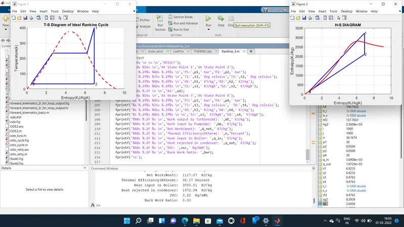
Output In Command Window

     

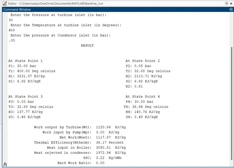
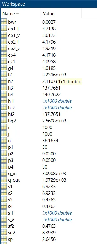
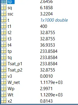
Screenshots Of The Output Screen 

ERRORS FACED WHILE PROGRAMMING

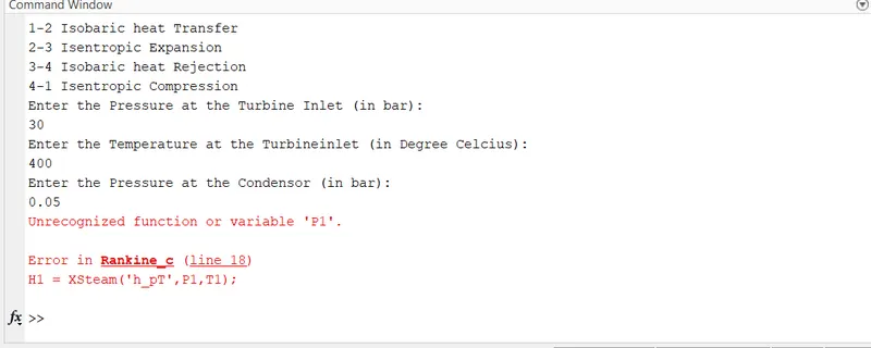
There are several errors faced and the main error is the variable recoganision. 

This error is cleared by giving the input variable and defining it

RESULT:

Hence, thermodynamic analysis of Rankine cycle was done successfully.

Thermal efficiency for given inputs of the Rankine cycle was found to be 36.17%.

Lowering the operating pressure of the condenser automatically lowers the temperature of the steam, and thus the temperature at which heat is rejected and hence thermal efficiency of the cycle increases.

Superheating of steam to a higher temperature results in overall increase in thermal efficiency.

References:

RANKINE POWER GENERATION CYCLE (colorado.edu)

Rankine Cycle PDF | PDF | Steam Engine | Steam (scribd.com)

Rankine Cycle (Steam Turbine) - MATLAB & Simulink - MathWorks India

Specific Steam Consumption - an overview | ScienceDirect Topics