Week 4.1 - Genetic Algorithm
Here we are creating the coding for get to optimise the stalagmite function and find the global maxima of the function.
We start our programe as usally we start with
clear all
close all
clc
Then we start giving the input values and first we assign x and y to take the values from 0-0.6 and want to have 150 values in between them too
And a variable num_case and give it value of 50
%input
x=linspace(0,0.6,150);
y=linspace(0,0.6,150);
num_case=50
now we want to create a 3D plot, we take a 2D array
%forming 2d array
[xx,yy]=meshgrid(x,y);
Here we create a 2D array of x and y using of meshgrid command and store its value in array then create an for loop to take the values stored in the array
for i=1:length(x)
for j=1:length(y)
input_vector(1)=xx(i,j);
input_vector(2)=yy(i,j);
then we read the values of array in to thr input_vectors(1)and input_vector(2)
f(i,j)=stagalmite(input_vector);
then we creat an another fuction with help of stalagmite function.the output that get from input_vectors are saved in to f(i,j) the fuction help us to get automatically maximum value
WE NEED TO CREATE FUNCTION IN ANOTHER FILE TO MINIMISE THE PROGRAME DIFFICULTY
We now creating an fuction named stagalmite and its saved in the same name ,if does not save in same name we will not get access the fuction when we call it in our main program
function A=stagalmite(input_vector)
it is the fuction we had create and the value of input_vector is read by the function from our main programme
x=input_vector(1);
y=input_vector(2);
then we are started assing of the x and y valued from the input_vector
Then we are creating the fuction main body part with help of the
F(x,y)=f1,xf2,xf1,yf2,y
f1,x=(sin(5.1*pi*x+0.5)).^6
f1,y=(sin(5.1*pi*y+0.5)).^6
f2,x= exp((-4*ln(2)*((x-0.0667).^2))/0.64)
f2,y=((-4*ln(2)*((y-0.0667).^2))/0.64)
for making the coding we change name of f,x and f,y to f1 ,f2 ,f3,f4 and introduce the eqution above derived to it
f1=(sin(5.1*pi*x+0.5)).^6;
f2=exp((-4*log(2)*((x-0.0667).^2))/0.64);
f3=(sin(5.1*pi*y+0.5)).^6;
f4=exp((-4*log(2)*((y-0.0667).^2))/0.64);
Then we are multiplying the values of f1,f2,f3,f4 as we see in the equtions above first line told
A=(f1*f2*f3*f4);
THE COMPLETE FUNCTION CALLING CODING IS
function A=stagalmite(input_vector)
x=input_vector(1);
y=input_vector(2);
f1=(sin(5.1*pi*x+0.5)).^6;
f2=exp((-4*log(2)*((x-0.0667).^2))/0.64);
f3=(sin(5.1*pi*y+0.5)).^6;
f4=exp((-4*log(2)*((y-0.0667).^2))/0.64);
A=(f1*f2*f3*f4);

end
After creating the function separate file saved we move to our main coding
Then we create for loop to the maximum value with help of stagalmite function to a array and reading the values in the array to xopt(i) and yopt(i)
%study 1 satistical behaviour
tic
for i=1:num_case
[inputs,fopt(i)]=ga(@stagalmite,2)
xopt(i)=inputs(1)
yopt(i)=inputs(2)
end
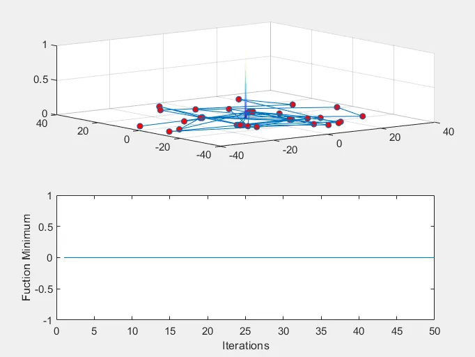
with the help above value we are creating the 3D plot
study_time1=toc
figure(1)
subplot(2,1,1)
surfc(x,y,f)
shading interp
hold on
plot3(xopt,yopt,fopt,'Marker','o','MarkerSize',5,'MarkerFaceColor','r')
subplot(2,1,2)
plot(fopt)
xlabel('Iterations')
ylabel('Fuction Minimum')
The output plot will be
%study 2 -stattistical behaviour -with upper and lower bond
As above we done ,we are creating another array too for saving the new values to xopt and yopt
tic
for i=1:num_case
[inputs,fopt(i)]=ga(@stagalmite,2,[],[],[],[],[0;0],[1;1]);
xopt(i)=inputs(1);
yopt(i)=inputs(2);
end
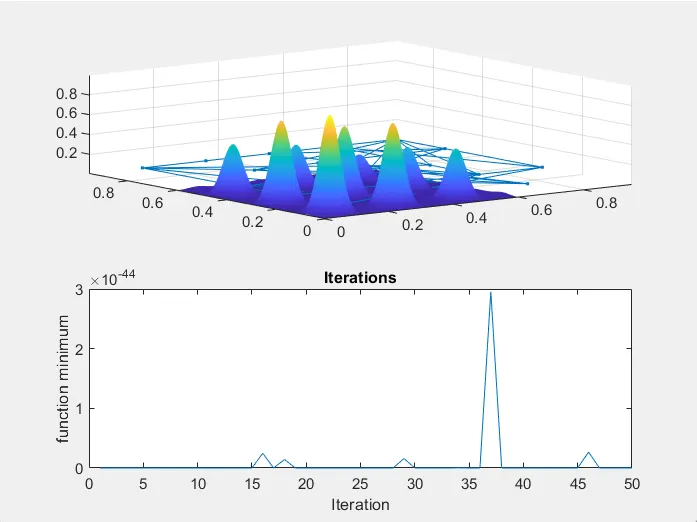
We use the plot3 command to make a plot of xopy,yopt,fopy to plot the optimum maximas and with the help of tic and toc commands we get the time taken to complete cycle we used
study_time2=toc
figure(2)
subplot(2,1,1)
surfc(x,y,f)
shading interp
hold on
plot3(xopt,yopt,fopt,'Marker','.','MarkerSize',5,'MarkerFaceColor','r')
subplot(2,1,2)
plot(fopt)
title('Iterations')
xlabel('Iteration')
ylabel('function minimum')
The out put plot for this will be as
Now we are pointing the down part and top part of x and y ,the ga is initiated with random population
for i=num_case
[inputs,fopt(i)]=ga(@stagalmite,2,[],[],[],[],[0;0],[1;1],[],[],options);
xopt(i)=inputs(1);
yopt(i)=inputs(2);
the output values that we had get grom the new loop are saved in the xopt and yopt
end
study_time3=toc
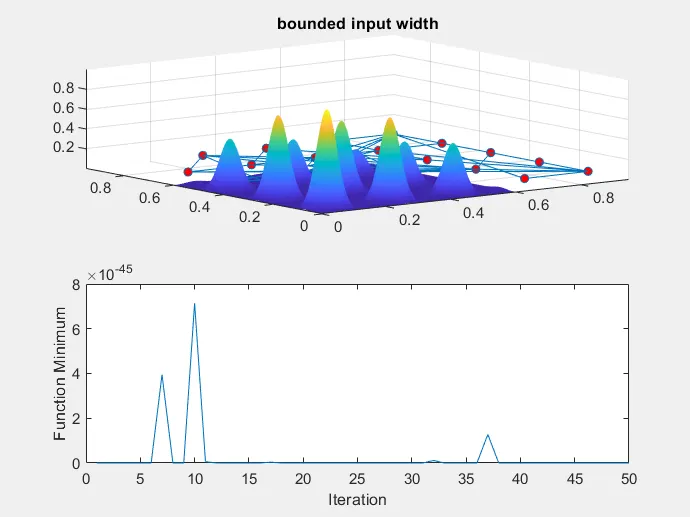
now we are starting t0 plot our third graph.We use the plot3 command to make a plot of xopy,yopt,fopy to plot the optimum maximas and with the help of tic and toc commands to record the time we get the time taken to complete cycle we used
and also we plot the graph of fopt function for getting the iteration
figure(3)
subplot(2,1,1)
surfc(x,y,f)
shading interp
hold on
plot3(xopt,yopt,fopt,'Marker','o','MarkerSize',5,'MarkerFaceColor','r')
title('bounded input width')
subplot(2,1,2)
plot(fopt)
xlabel('Iteration')
ylabel('Function Minimum')
THE PLOT AS RESULT WE GET IS
THE COMPLETE CODING FOR GETTING THE ABOVE ALL CODING IS
clear all
close all
clc

%input
x=linspace(0,0.6,150);
y=linspace(0,0.6,150);
num_case=50

%forming 2d array
[xx,yy]=meshgrid(x,y);
for i=1:length(x)
    for j=1:length(y)
        input_vector(1)=xx(i,j);
         input_vector(2)=yy(i,j);
         f(i,j)=stagalmite(input_vector);
    end
end

%study 1  satistical behaviour
tic
for i=1:num_case
    [inputs,fopt(i)]=ga(@stagalmite,2)
    xopt(i)=inputs(1)
    yopt(i)=inputs(2)
end
study_time1=toc
figure(1)
subplot(2,1,1)
surf(x,y,f)
shading interp
hold on
plot3(xopt,yopt,fopt,'Marker','o','MarkerSize',5,'MarkerFaceColor','r')
subplot(2,1,2)
plot(fopt)
xlabel('Iterations')
ylabel('Fuction Minimum')

%study 2 -stattistical behaviour -with upper and lower bomds
tic
for i=1:num_case
    [inputs,fopt(i)]=ga(@stagalmite,2,[],[],[],[],[0;0],[1;1]);
    xopt(i)=inputs(1);
    yopt(i)=inputs(2);
end

study_time2=toc

figure(2)
subplot(2,1,1)
surfc(x,y,f)
shading interp
hold on
plot3(xopt,yopt,fopt,'Marker','.','MarkerSize',5,'MarkerFaceColor','r')
subplot(2,1,2)
plot(fopt)
title('Iterations')
xlabel('Iteration')
ylabel('function minimum')

%study 3 increasing ga iterations
tic
options=optimoptions('ga');
options=optimoptions(options,'populationsize',250);

for i=num_case
    [inputs,fopt(i)]=ga(@stagalmite,2,[],[],[],[],[0;0],[1;1],[],[],options);
    xopt(i)=inputs(1);
    yopt(i)=inputs(2);
end
study_time3=toc
figure(3)
subplot(2,1,1)
surfc(x,y,f)
shading interp
hold on
plot3(xopt,yopt,fopt,'Marker','o','MarkerSize',5,'MarkerFaceColor','r')
title('bounded input width')
subplot(2,1,2)
plot(fopt)
xlabel('Iteration')
ylabel('Function Minimum')