Project 2 - Rankine cycle Simulator
Here we are creating the coding to find out the Rankine Cycle Simulator using our MAT Lab and the required values that we want to assing in the calculation section are given in the challenge
Required Inputs:
Turbine Inlet temperature = 400° C
Turbine Inlet Pressure = 30 bars
Turbine Outlet Pressure = 0.05 bars = Condenser Inlet Pressure
We will start our coding as we do all other coding with
clear all
close all
clc
subscript for different state points
1=Turbine inlet or Boiler outlet
2=Condenser inlet or Turbine outlet
3=Pump inlet or condenser outlet ,4=Boiler inlet or pump outlet
Input parameters-
P1=Turbine inlet pressure (bar)
T1=Temperature at turbine inlet(deg c),
P2=Turbine outlet pressure (bar)
Here we are printing the description about four process, if we does not the semi column we see that the below wrinten things under the bracket will display in pur comment box
fprintf('process (1-2)-Isentropic Expansion in the Turbine');
fprintf('process (2-3)-Isobaric Heat Rejection by the Condenser');
fprintf('process (3-2)-Isentropic Compression in the pump');
fprintf('process (4-1)-Isobaric Heat Addition by the Boiler');
To get different state variables,all the process parameters should be Expressed such as all four process occure and input parameters as state 1
p1=input('Enter the pressure at the Turbine Inlet (in bar):');
t1=input('Enter the Temperature at the aturbine inlet (in Degree celsius:');
p2=input('Enter the Pressure at the Turbine Outlet (in bar):');
from the standard XSteam library that we get from the link provided in the challenge section to get the steam table data for water ,most of the point in between state variables are calculated .And their corresponding parameters such as enthalpy ,entropy,specific heat ,saturation temperature ,etc
h1=XSteam('h_pT',p1,t1);
Enthalpy in [KJ/Kg]
s1=XSteam('s_pT',p1,t1);
specific entropy in [KJ/Kg k]
v1=XSteam('v_pT',p1,t1);
specific volume in [m3/kg]
All the state points are used to find our net work done by turbine, thermal efficiency ,back work ratio ,etc according to their thermodynamic relations and necessary formulas
State 2,variable at condenser inlet
s2=s1;
Specific entropy in {KJ/Kg K]
h2=XSteam('h_px',p2,XSteam('x_ps',p2,s2));
Enthalpy in [KJ/Kg]
t2=XSteam('T_ps',p2,s2);
Tempereture in [degree C]
v2=XSteam('v_ps',p2,s2);
SPecific volume in [m3/Kg]
state 3,variable at pump inlet
p3=p2; %Pressure in [bar]
t3=XSteam('Tsat_p',p3); %Temperature in [degree C]
h3=XSteam('hL_p',p3); %Enthalpy in [KJ/Kg]
s3=XSteam('sL_p',p3); %Specific entropy in [KJ/Kf K]
v3=XSteam('vL_p',p3); %Inlet Specific volume in [m3/Kg]
%state 4,variable at Boiler Inlet
s4=s3; %Specific entropy in [kKJ/Kg K]
p4=p1; %Pressure in [bar]
h4=XSteam('h_ps',p4,s4); %Enthalpy in [KJ/Kg]
t4=XSteam('T_ps',p4,s4); %Temperature in [degree C]
v4=XSteam('v_ps',p4,s4); %Specific volume in [m3/Kg]
after defining all states now lets process each these states and in between data variable
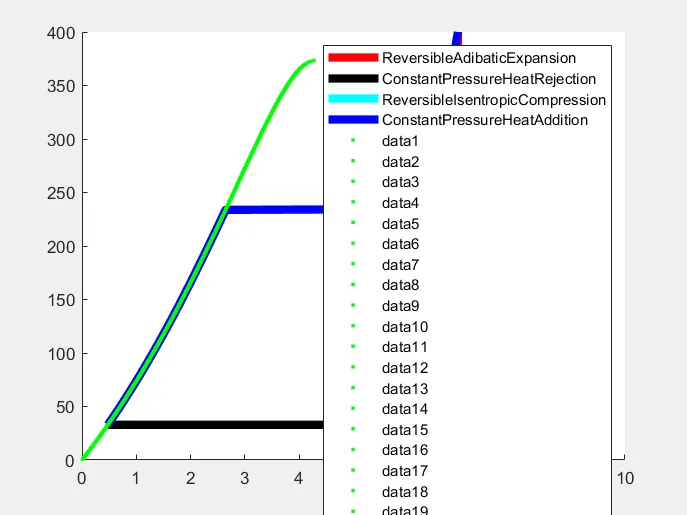
To plot the property diagram of water ,i.e.,saturation liquid and vapour line ,an array is created using linspace command from 0 to values of t1 with 5000 evenly spaced points in between them and suitable state variable are iterated using for loop .
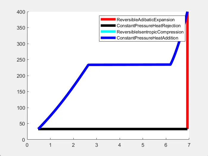
plotting Graph for Ideal Rankine cycle in "T" vs "s"
figure(1)
hold on
plot([s1 s2],[t1 t2],'Color','r','LineWidth',5);
plot([s2 s3],[t2 t3],'Color','k','LineWidth',5);
plot([s3 s4],[t3 t4],'Color','c','LineWidth',5);
Trange=linspace(t4,t1,500);
for i=1:length(Trange)
s_range(i)=XSteam('s_pt',p1,Trange(i));
h_range23(i)=XSteam('h_ps',p1,s_range(i));
h_range41(i)=XSteam('h_ps',p2,s_range(i));
end
plot(s_range,Trange,'color','b','LineWidth',5);
legend('ReversibleAdibaticExpansion','ConstantPressureHeatRejection','ReversibleIsentropicCompression','ConstantPressureHeatAddition');
to plot t-s and h-s diagram ,all required points are ploted and marked using text command
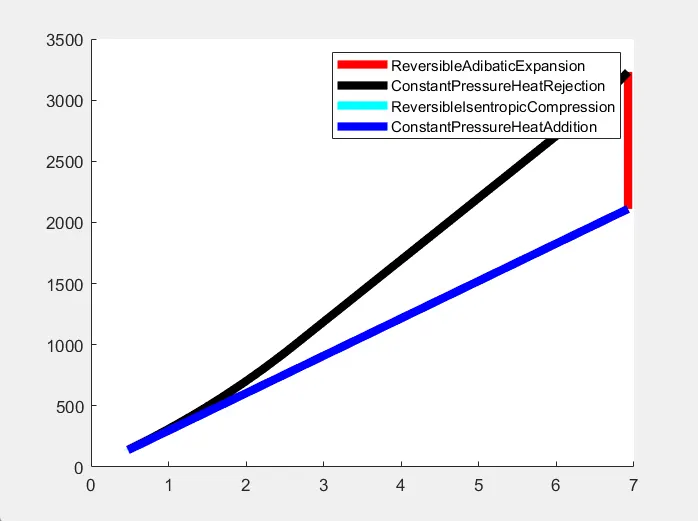
plotting Graph FOr Ideal Rankine Cycle in 'h' vs 's'
figure(2)
hold on
plot([s1 s2],[h1 h2],'Color','r','LineWidth',5);
plot(s_range,h_range23,'Color','k','LineWidth',5);
plot([s3 s4],[h3 h4],'Color','c','LineWidth',5);
plot(s_range,h_range41,'Color','b','LineWidth',5);
legend('ReversibleAdibaticExpansion','ConstantPressureHeatRejection','ReversibleIsentropicCompression','ConstantPressureHeatAddition');
plotting graph for 'T' vs 's'
t_range=linspace(0,374.15,500);
temperature from 0 to critical pointof water in [degree c]
figure(1)
hold on
for i=1:length(t_range)
plot(XSteam('sL_t',t_range(i)),t_range(i),'.','Color','g')
plot(XSteam('sV_t',t_range(i)),t_range(i),'.','Color','g')
end
ploting graphs for 'h' vs 's'
figure(2)
hold on
for i=1:length(t_range)
plot(XSteam('sL_t',t_range(i)),XSteam('hL_t',t_range(i)),'.','Color','g')
plot(XSteam('sV_t',t_range(i)),XSteam('hL_t',t_range(i)),'.','Color','g')
end
ploting diagram for all state point for Ideal Rankine cycle in 'T' vs 's'
figure(1)
hold on
plot(s1,t1,'ko')
plot(s2,t2,'ko')
plot(s3,t3,'ko')
plot(s4,t4,'ko')
grid on
title('T-s Diagram of RANKINE CYCLE')
xlabel('Temperature in [degree C]')
ylabel('Specific entropy in [KJ/kg K]')
Plotting Diagram for all state point for Ideal Rankine cycle in 'h' vs 's'
figure(2)
hold on
plot(s1,h1,'ko')
plot(s2,h2,'ko')
plot(s3,h3,'ko')
plot(s4,h4,'ko')
grid on
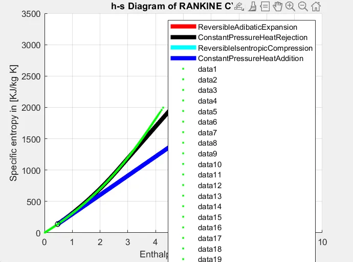
title('h-s Diagram of RANKINE CYCLE')
xlabel('Enthalpy in [KJ/Kg K]')
ylabel('Specific entropy in [KJ/kg K]')
Finally calculating Work and Efficiency
Work_turbine=h1-h2;
work transferred from the working fluid(KJ/Kg)
Q_taken_out_condenser=h2-h3;
heat rejected from the working fluid (KJ/Kg)
Work_pump=h4-h3; %
work transferred into the working fluid (KJ/Kg)
Q_given_boiler=h1-h4;
heat transferred to the working fluid (KJ/Kg)
Back_work_Ratio=Work_turbine/Work_pump;
SSE=3600/(Work_turbine-Work_pump);
specific steam cosumption [kg/kwh]
Work_net=Work_turbine-Work_pump;
Net work on the work fuid (KJ/Kg)
Effi_rankine=Work_net/Q_given_boiler;
Rankine Cycle Efficiency
Clc
printing results to the USER GIVING input
fprintf('**********RANKINE CYCLE:IDEAL CYCLE FOR VAPOUR POWER CYCLE**********nn')
fprintf('process 1-2:Reversible adiabati expansion process in the steam turbine');
fprintf('process 2-3:Constant pressure heat trensfer process in the condenser');
fprintf('process 3-4:Reversible adiabatic compression process in the pump');
fprintf('process 4-1:Constant pressure heat transfer process in the boiler');
fprintf('----------State variable at state point 1----------n');
fprintf('Turbine Inlet Temperature T!=%.5f in[degree c]n',t1);
fprintf('Turbine Inlet pressure p1=%.5f in [bar]n',p1);
fprintf('Turbine Inlet Enthalpy h1=%.5f in [KJ/Kg]n',h1);
fprintf('Turbine Inlet specific entropy s1=%.5f in [KJ/Kg k]n',s1);
fprintf('Turbine Inlet specific volume v1=%.5f in [m3/Kg]nn',v1);
fprintf('----------State variable at state point 2----------n');
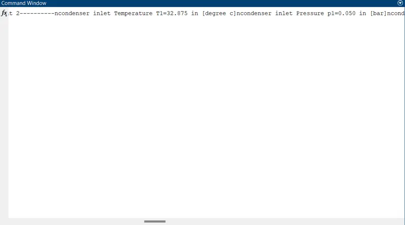
fprintf('condenser inlet Temperature T1=%.3f in [degree c]n',t2);
fprintf('condenser inlet Pressure p1=%.3f in [bar]n',p2);
fprintf('condenser inlet Enthalpy h1=%.3f in [KJ/Kg]n',h2);
fprintf('condenser inlet specific entropy s1=%.3f in [KJ/Kg k]n',s2);
fprintf('condenser inlet specific volume v1=%.3f in [m3/Kg]nn',v2);
fprintf('----------State variable at state point 3----------n');
fprintf('pump inlet temperature T1=%.3f in [degree c]n',t3);
fprintf('pump inlet pressure p1=%.3f in [bar]n',p3);
fprintf('pump inlet Enthalpy h1=%.3f in [KJ/Kg]n',h3)
fprintf('pump inlet specific entropy s1=%.3f in [KJ/Kg K]n',s3);
fprintf('pump inlet specific volume v1=%.3f in [m3/Kg]nn',v3);
fprintf('----------State variable at state point 4----------n');
fprintf('boiler inlet Temperature T1=%.4f in [degree c]n',t4);
fprintf('boiler inlet pressure p1=%.3f in [bar]n',p4);
fprintf('boiler inlet Enthalpy h1=%.3f in [KJ/Kg]n',h4)
fprintf('boiler inlet specific entropy s1=%.3f in [KJ/Kg K]n',s4);
fprintf('boiler inlet specific volume v1=%.3f in [m3/Kg]nn',v4);
fprintf('----------Work and Efficieny----------n');
fprintf('Work transferred from the working fluid Wturbine=%.4f in [KJ/Kg]n',Work_turbine);
fprintf('Heat rejected from the working fluid Qcondenser=%.4f in [KJ/Kg]n',Q_taken_out_condenser);
fprintf('Work transferred into the Working fluid Wpump=%.4f in [KJ/Kg]n',Work_pump);
fprintf('Heat transferred to the working fluid Qboiler=%.4f in [KJ/Kg]n',Q_given_boiler)
fprintf('Back Work Ratio BWR=%.4f n',Back_work_Ratio);
fprintf('Specific Steam Consumption SSE=%.4f in [Kg/kwh]n',SSE);
fprintf('Rankine Cycle Efficiency ETArankine=%.4f%%nn',Effi_rankine*100);
fprintf('n............... SUCESSFULLY DONE THE CALCULATIONS...............n');
THE COMPLETE CODING IS
clear all
close all
clc

%subscript for different state points
%1=Turbine inlet or Boiler outlet, 2=Condenser inlet or Turbine outlet
%,3=Pump inlet or condenser outlet ,4=Boiler inlet or pump outlet
%Input parameters-
%P1=Turbine inlet pressure (bar)
%T1=Temperature at turbine inlet(deg c),
%P2=Turbine outlet pressure (bar)
%description about four process,
fprintf('process (1-2)-Isentropic Expansion in the Turbine');
fprintf('process (2-3)-Isobaric Heat Rejection by the Condenser');
fprintf('process (3-2)-Isentropic Compression in the pump');
fprintf('process (4-1)-Isobaric Heat Addition by the Boiler');

%for Input state variable at ponit 1
p1=input('Enter the pressure at the Turbine Inlet (in bar):');
t1=input('Enter the Temperature at the aturbine inlet (in Degree celsius:');
p2=input('Enter the Pressure at the Turbine Outlet (in bar):');

%state variable at Turbian Inlet
h1=XSteam('h_pT',p1,t1);                    %Enthalpy in [KJ/Kg]
s1=XSteam('s_pT',p1,t1);                    %specific entropy in [KJ/Kg k]
v1=XSteam('v_pT',p1,t1);                    %specific volume in [m3/kg]

%State variable at condenser inlet

s2=s1;                                      %Specific entropy in {KJ/Kg K]
h2=XSteam('h_px',p2,XSteam('x_ps',p2,s2));  %Enthalpy in [KJ/Kg]
t2=XSteam('T_ps',p2,s2);                    %Tempereture in [degree C]
v2=XSteam('v_ps',p2,s2);                    %SPecific volume in [m3/Kg]

%state variable at pump inlet

p3=p2;                                      %Pressure in [bar]
t3=XSteam('Tsat_p',p3);                     %Temperature in [degree C]
h3=XSteam('hL_p',p3);                       %Enthalpy in [KJ/Kg]
s3=XSteam('sL_p',p3);                       %Specific entropy in [KJ/Kf K]
v3=XSteam('vL_p',p3);                       %Inlet Specific volume in [m3/Kg]

%state variable at Boiler Inlet

s4=s3;                                      %Specific entropy in [kKJ/Kg K]
p4=p1;                                      %Pressure in [bar]
h4=XSteam('h_ps',p4,s4);                    %Enthalpy in [KJ/Kg]
t4=XSteam('T_ps',p4,s4);                    %Temperature in [degree C]
v4=XSteam('v_ps',p4,s4);                    %Specific volume in [m3/Kg]

%after defining all states now lets process each  these states and in between data variable

%plotting Graph for Ideal Rankine cycle in "T" vs "s"

figure(1)
hold on
plot([s1 s2],[t1 t2],'Color','r','LineWidth',5);
plot([s2 s3],[t2 t3],'Color','k','LineWidth',5);
plot([s3 s4],[t3 t4],'Color','c','LineWidth',5);
Trange=linspace(t4,t1,500);
for i=1:length(Trange)
    s_range(i)=XSteam('s_pt',p1,Trange(i));
    h_range23(i)=XSteam('h_ps',p1,s_range(i));
    h_range41(i)=XSteam('h_ps',p2,s_range(i));
end
plot(s_range,Trange,'color','b','LineWidth',5);
legend('ReversibleAdibaticExpansion','ConstantPressureHeatRejection','ReversibleIsentropicCompression','ConstantPressureHeatAddition');

%plotting Graph FOr Ideal Rankine Cycle in 'h' vs 's'
figure(2)
hold on
plot([s1 s2],[h1 h2],'Color','r','LineWidth',5);
plot(s_range,h_range23,'Color','k','LineWidth',5);
plot([s3 s4],[h3 h4],'Color','c','LineWidth',5);
plot(s_range,h_range41,'Color','b','LineWidth',5);
legend('ReversibleAdibaticExpansion','ConstantPressureHeatRejection','ReversibleIsentropicCompression','ConstantPressureHeatAddition');

%plotting graph for 'T' vs 's'
t_range=linspace(0,374.15,500);             %temperature from 0 to critical pointof water in [degree c]
figure(1)
hold on
for i=1:length(t_range)
    plot(XSteam('sL_t',t_range(i)),t_range(i),'.','Color','g')
    plot(XSteam('sV_t',t_range(i)),t_range(i),'.','Color','g')
end

%ploting graphs for 'h' vs 's'
figure(2)
hold on
for i=1:length(t_range)
    plot(XSteam('sL_t',t_range(i)),XSteam('hL_t',t_range(i)),'.','Color','g')
    plot(XSteam('sV_t',t_range(i)),XSteam('hL_t',t_range(i)),'.','Color','g')
end

%ploting diagram for all state point for Ideal Rankine cycle in 'T' vs 's'
figure(1)
hold on
plot(s1,t1,'ko')
plot(s2,t2,'ko')
plot(s3,t3,'ko')
plot(s4,t4,'ko')
grid on
title('T-s Diagram of RANKINE CYCLE')
xlabel('Temperature in [degree C]')
ylabel('Specific entropy in [KJ/kg K]')

%Plotting Diagram for all state point for Ideal Rankine cycle in 'h' vs 's'
figure(2)
hold on
plot(s1,h1,'ko')
plot(s2,h2,'ko')
plot(s3,h3,'ko')
plot(s4,h4,'ko')
grid on
title('h-s Diagram of RANKINE CYCLE')
xlabel('Enthalpy in [KJ/Kg K]')
ylabel('Specific entropy in [KJ/kg K]')

%Finally calculating Work and Efficiency

Work_turbine=h1-h2;            %work transferred from the working fluid(KJ/Kg)
Q_taken_out_condenser=h2-h3;   %heat rejected from the working fluid (KJ/Kg)
Work_pump=h4-h3;               %work transferred into the working fluid (KJ/Kg)
Q_given_boiler=h1-h4;          %heat transferred to the working fluid (KJ/Kg)
Back_work_Ratio=Work_turbine/Work_pump;
SSE=3600/(Work_turbine-Work_pump);    %specific steam cosumption [kg/kwh]
Work_net=Work_turbine-Work_pump;      %Net work on the work fuid (KJ/Kg)
Effi_rankine=Work_net/Q_given_boiler; %Rankine Cycle Efficiency

clc
%printing results to the USER GIVING input
fprintf('**********RANKINE CYCLE:IDEAL CYCLE FOR VAPOUR POWER CYCLE**********nn')
fprintf('process 1-2:Reversible adiabati expansion process in the steam turbine');
fprintf('process 2-3:Constant pressure heat trensfer process in the condenser');
fprintf('process 3-4:Reversible adiabatic compression process in the pump');
fprintf('process 4-1:Constant pressure heat transfer process in the boiler');
fprintf('----------State variable at state point 1----------n');
fprintf('Turbine Inlet Temperature T!=%.5f in[degree c]n',t1);
fprintf('Turbine Inlet pressure p1=%.5f in [bar]n',p1);
fprintf('Turbine Inlet Enthalpy h1=%.5f in [KJ/Kg]n',h1);
fprintf('Turbine Inlet specific entropy s1=%.5f in [KJ/Kg k]n',s1);
fprintf('Turbine Inlet specific volume v1=%.5f in [m3/Kg]nn',v1);

fprintf('----------State variable at state point 2----------n');
fprintf('condenser inlet Temperature T1=%.3f in [degree c]n',t2);
fprintf('condenser inlet Pressure p1=%.3f in [bar]n',p2);
fprintf('condenser inlet Enthalpy h1=%.3f in [KJ/Kg]n',h2);
fprintf('condenser inlet specific entropy s1=%.3f in [KJ/Kg k]n',s2);
fprintf('condenser inlet specific volume v1=%.3f in [m3/Kg]nn',v2);

fprintf('----------State variable at state point 3----------n');
fprintf('pump inlet temperature T1=%.3f in [degree c]n',t3);
fprintf('pump inlet pressure p1=%.3f in [bar]n',p3);
fprintf('pump inlet Enthalpy h1=%.3f in [KJ/Kg]n',h3)
fprintf('pump inlet specific entropy s1=%.3f in [KJ/Kg K]n',s3);
fprintf('pump inlet specific volume v1=%.3f in [m3/Kg]nn',v3);

fprintf('----------State variable at state point 4----------n');
fprintf('boiler inlet Temperature T1=%.4f in [degree c]n',t4);
fprintf('boiler inlet pressure p1=%.3f in [bar]n',p4);
fprintf('boiler inlet Enthalpy h1=%.3f in [KJ/Kg]n',h4)
fprintf('boiler inlet specific entropy s1=%.3f in [KJ/Kg K]n',s4);
fprintf('boiler inlet specific volume v1=%.3f in [m3/Kg]nn',v4);

fprintf('----------Work and Efficieny----------n');
fprintf('Work transferred from the working fluid Wturbine=%.4f in [KJ/Kg]n',Work_turbine);
fprintf('Heat rejected from the working fluid Qcondenser=%.4f in [KJ/Kg]n',Q_taken_out_condenser);
fprintf('Work transferred into the Working fluid Wpump=%.4f in [KJ/Kg]n',Work_pump);
fprintf('Heat transferred to the working fluid Qboiler=%.4f in [KJ/Kg]n',Q_given_boiler)

fprintf('Back Work Ratio BWR=%.4f n',Back_work_Ratio);
fprintf('Specific Steam Consumption SSE=%.4f in [Kg/kwh]n',SSE);
fprintf('Rankine Cycle Efficiency ETArankine=%.4f%%nn',Effi_rankine*100);

fprintf('n............... SUCESSFULLY DONE THE CALCULATIONS...............n');
%%end
THE OUTPUT GRAPH ARE WILL BE
THE OUTPUT IN COMMAND WINDOW IS