Project 1 - Parsing NASA thermodynamic data
In this coding we accually reading the data or value from an another file and taking access to the line or one fixed point’s value for read and write that values to our coding with the help of commands like
fopen – to open a data files full values and text present in to our coding
fprint – to add any text or value to saved file or document
fclose – is used after doing fprint operation ,its done for stoping the printing option
tline – its runs the file to getting the details of variable
We start our program as usually we start with
clear all
close all
clc
For opening first we need to open or download the file its named as THERMO in our programesave that file in the location in where we had saved the coding files too.Then with the help of fopen command we read all text and value of the document and read the values in to a variable and we named it as ‘f1’
f1=fopen('THERMO.dat','r');
fget here is used to read one line of text from the instrument connected to f1 ,and returns the data
fgetl(f1);
Now we want to read the values of temperature from the data for our calculations
Then first value of temperature is converted with the help of string2number (str2num) command so that the no in “ can be converted into plain number.
temp=str2num(fgetl(f1));
now we have assigned temperatures to the global low temperature ,global medium temperature,high temperature
global_low_temp=temp(1);
global_mid_temp=temp(2);
global_high_temp=temp(3);
Now as shown in when exicute the program we get so many unwanted line in figure for removing those line we use a loop 1:3 means avoiding or skip these 3 lines
for i=1:3
fgetl(f1);
end
reading the header information
for i=1:4:212
tline=fgetl(f1)
To split the given value in line we have used strsplit and then we calculate the species value
a=strsplit(tline,' ');
b=length(a);
species=a{1};
Then we are converting local temperature into double precision value and to convert the complex number into cell array/string array we will use str2double command
low_temp=str2double(a(b-3));
mid_temp=str2double(a(b-2));
high_temp=str2double(a(b-1));
Then we are storing the values in the second line of variable we use fgetl command here also but assing to the line from to which we want to get the values
line2=fgetl(f1);
To find the value(string) of thst particular line now we will use strfind command
c=strfind(line2,'E');
then we use str2double we will find 14 coefficient and next 7 are lower temperature
a1=str2double(line2(1:(c(1)+3)));
a2=str2double(line2((c(1)+4):(c(2)+3)));
a3=str2double(line2((c(2)+4):(c(3)+3)));
a4=str2double(line2((c(3)+4):(c(4)+3)));
a5=str2double(line2((c(3)+4):(c(5)+3)));
As above same process are repeated to fined the lines 3 and 4too
line3=fgetl(f1);
Here we find the position of the expontion
d=strfind(line3,'E');
a6=str2double(line3(1:(d(1)+3)));
a7=str2double(line3((d(1)+4):(d(2)+3)));
a8=str2double(line3((d(2)+4):(d(3)+3)));
a9=str2double(line3((d(3)+4):(d(4)+3)));
a10=str2double(line3((d(4)+4):(d(5)+3)));
line4=fgetl(f1);
e=strfind(line4,'E');
a11=str2double(line4(1:(e(1)+3)));
a12=str2double(line4((e(1)+4):(e(2)+3)));
a13=str2double(line4((e(2)+4):(e(3)+3)));
a14=str2double(line4((e(3)+4):(e(4)+3)));
Then we will define the higher and lower temperatures with help of linspace comment and the temperature range are too we are defining
lower_temp=linspace(low_temp,mid_temp,100)
higher_temp=linspace(mid_temp,high_temp,100)
then we are assuming the universal gas costant R as 8.134j/mol^-k and
R=8.314;
Then after giving all values of a in respective commands of enthalpy, entropy, and specific heat we want to plot the graph
Lower temperature values for cp,h,s and eqution to find them are

cp_low(k)=(a8+(a9*lower_temp(k))+(a10*(lower_temp(k)^2)+(a11*lower_temp(k))^3)+a12*(lower_temp(k)^4))*R;
h_low(k)=(a8+(a9*lower_temp(k))/2+(a10*lower_temp(k)^2)/3+(a11*lower_temp(k)^3)/4+a12*(lower_temp(k)^4)/5+(a13/lower_temp(k)))*R*lower_temp(k);
s_low(k)=((a8*log(lower_temp(k))+(a9*lower_temp(k))+((a10*lower_temp(k)^2)/2)+((a11*lower_temp(k)^3)/3)+((a12*lower_temp(k)^4)/4)+a14)*R);
higher temperature values for cp,h,s
cp_high(k)=(a1+(a2*higher_temp(k))/2+(a3*higher_temp(k)^2)/3+(a4*higher_temp(k)^3)/4+(a5*(higher_temp(k)^4))/5+(a6/higher_temp(k)))*R*higher_temp(k);
h_high(k)=(a1+(a2*higher_temp(k))/2+(a3*higher_temp(k)^2)/3+(a4*higher_temp(k)^3)/4+(a5*(higher_temp(k)^4))/5+(a6/higher_temp(k)))*R*higher_temp(k);
s_high(k)=((a1*log(higher_temp(k))+a2*higher_temp(k)+((a3*higher_temp(k)^2)/2)+((a4*higher_temp(k)^3)/3)+((a5*higher_temp(k)^4)/4)+a7)*R);
end
to do the plotting coding we want to make folder for saving the plots so the current_drive=pwd opens present working directory and the mkdir command makes the new folder with the name specified inside bracket
nasa_garphs=species;
mkdir(nasa_garphs);
current=pwd;
cd(nasa_garphs);
command cd makes new folder as directory which is used for storing al related output file of the program
then we are plotting the graphs as required and with the values that we obtained from above all
%specific heat
figure(1)
plot(lower_temp,cp_low,'LineWidth',3)
hold on
plot(higher_temp,cp_high,'LineWidth',3)
hold off
title(['TEMPURATURE VS SPECIFIC HEAT',species])
xlabel('TEMPERTURE');
ylabel('SPECIFIC HEAT');
legend('Low Temperature','High Temperatute');
fig=sprintf('Specific Heat of %s.png',species);
saveas(gca,fig);
%For Enthalpy
figure(2)
plot(lower_temp,h_low,'LineWidth',3)
hold on
plot(higher_temp,h_high,'LineWidth',3)
hold off
title(['Tempurature vs Entalpy',species])
xlabel('TEMPURTURE')
ylabel('ENTALPY')
legend('low Temperature','high Temperature')
fig=sprintf('Enthalpy of %s.png',species);
saveas(gca,fig);
%for entropy
figure(3)
plot(lower_temp,s_low,'LineWidth',3)
hold on
plot(higher_temp,s_high,'LineWidth',3)
hold off
title(['Temperature vs Entropy',species])
xlabel('Temperture')
ylabel('Entropy')
legend('low temperature','high temperature');
fig=sprintf('Entropy of %s.png',species);
saveas(gca,fig);
cd(current)
end
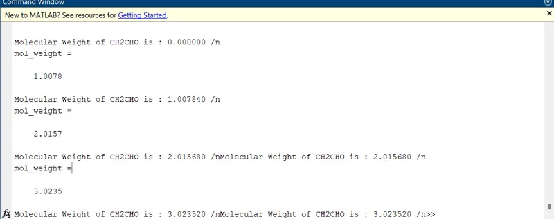
%Calculating Molecular weight
atoms=['H','C','N','R','S'];
atom_weight=[1.00784 12.0109 16.002 39.065 32.067]
mol_weight=0;
species_check=char(species);
for i=1:length(species_check)
for j=1:length(atom)
if(strcmp(species_check(i),atoms(j)))
mol_weight=mol_weight+atom_weight(j)
position=j;
end
end
x=str2double(species_check(i));
if x>1
mol_weight=mol_weight+(atom_weight(j)*(x-1))
end
fprintf('Molecular Weight of %s is : %f /n',species_check,mol_weight)
end
THE COMPELTE CODING FOR GETTING THE OUTPUT IS
clear all
close all
clc

f1=fopen('THERMO.dat','r');
fgetl(f1);

%for grtting temperture value

temp=str2num(fgetl(f1));
global_low_temp=temp(1);
global_mid_temp=temp(2);
global_high_temp=temp(3);

%for skipping unwanted lines
for i=1:3
    fgetl(f1);
end

%creating loop for all spicies that calculate data,plot graph and molecular weight


for i=1:4:212
    tline=fgetl(f1);

    a=strsplit(tline,' ');
    b=length(a);
    species=a{1};

%storing values of temperture

low_temp=str2double(a(b-3));
mid_temp=str2double(a(b-2));
high_temp=str2double(a(b-1));

%storing second line values

line2=fgetl(f1);%storing the value 2nd line in a veriable


%finding the position of E

c=strfind(line2,'E');

%creating individual coefficients

a1=str2double(line2(1:(c(1)+3)));
a2=str2double(line2((c(1)+4):(c(2)+3)));
a3=str2double(line2((c(2)+4):(c(3)+3)));
a4=str2double(line2((c(3)+4):(c(4)+3)));
a5=str2double(line2((c(3)+4):(c(5)+3)));

%storing the values of 3rd line

line3=fgetl(f1);

%finding position of E

d=strfind(line3,'E');

%storing the value in 3rd line
a6=str2double(line3(1:(d(1)+3)));
a7=str2double(line3((d(1)+4):(d(2)+3)));
a8=str2double(line3((d(2)+4):(d(3)+3)));
a9=str2double(line3((d(3)+4):(d(4)+3)));
a10=str2double(line3((d(4)+4):(d(5)+3)));

%storing the values of 2th line

line4=fgetl(f1);

%finding the postion of E

e=strfind(line4,'E');

%storing the values of fourth line

a11=str2double(line4(1:(e(1)+3)));
a12=str2double(line4((e(1)+4):(e(2)+3)));
a13=str2double(line4((e(2)+4):(e(3)+3)));
a14=str2double(line4((e(3)+4):(e(4)+3)));

% creating ranges for low amd high temperture
 lower_temp=linspace(low_temp,mid_temp,100)
 higher_temp=linspace(mid_temp,high_temp,100)

 %inputing the values of universal gas constant R=8.314 j/mol*k

 R=8.314;

 %calculating the values for Cp,H and S using the for loop given formula

 for k=1:100


 %lower temperature values for Cp,H,S
 cp_low(k)=(a8+(a9*lower_temp(k))+(a10*(lower_temp(k)^2)+(a11*lower_temp(k))^3)+a12*(lower_temp(k)^4))*R;
 h_low(k)=(a8+(a9*lower_temp(k))/2+(a10*lower_temp(k)^2)/3+(a11*lower_temp(k)^3)/4+a12*(lower_temp(k)^4)/5+(a13/lower_temp(k)))*R*lower_temp(k);
 s_low(k)=((a8*log(lower_temp(k))+(a9*lower_temp(k))+((a10*lower_temp(k)^2)/2)+((a11*lower_temp(k)^3)/3)+((a12*lower_temp(k)^4)/4)+a14)*R);

 %higher tempertyure values for cp,h,s

 cp_high(k)=(a1+(a2*higher_temp(k))/2+(a3*higher_temp(k)^2)/3+(a4*higher_temp(k)^3)/4+(a5*(higher_temp(k)^4))/5+(a6/higher_temp(k)))*R*higher_temp(k);
 h_high(k)=(a1+(a2*higher_temp(k))/2+(a3*higher_temp(k)^2)/3+(a4*higher_temp(k)^3)/4+(a5*(higher_temp(k)^4))/5+(a6/higher_temp(k)))*R*higher_temp(k);
 s_high(k)=((a1*log(higher_temp(k))+a2*higher_temp(k)+((a3*higher_temp(k)^2)/2)+((a4*higher_temp(k)^3)/3)+((a5*higher_temp(k)^4)/4)+a7)*R);
 end

 %making folder for saving the plots

 nasa_garphs=species;
 mkdir(nasa_garphs);
 current_dir=pwd;
 cd(nasa_garphs);

 %plotting graph

 %specific heat
 figure(1)
 plot(lower_temp,cp_low,'LineWidth',3)
 hold on
 plot(higher_temp,cp_high,'LineWidth',3)
 hold off
 title(['TEMPURATURE VS SPECIFIC HEAT',species])
 xlabel('TEMPERTURE');
 ylabel('SPECIFIC HEAT');
 legend('Low Temperature','High Temperatute');
 fig=sprintf('Specific Heat of %s.png',species);
 saveas(gca,fig);


 %For Enthalpy
 figure(2)
 plot(lower_temp,h_low,'LineWidth',3)
 hold on
 plot(higher_temp,h_high,'LineWidth',3)
 hold off
 title(['Tempurature vs Entalpy',species])
 xlabel('TEMPURTURE')
 ylabel('ENTALPY')
 legend('low Temperature','high Temperature')
 fig=sprintf('Enthalpy of %s.png',species);
 saveas(gca,fig);


 %for entropy
 figure(3)
 plot(lower_temp,s_low,'LineWidth',3)
 hold on
 plot(higher_temp,s_high,'LineWidth',3)
 hold off
 title(['Temperature vs Entropy',species])
 xlabel('Temperture')
 ylabel('Entropy')
 legend('low temperature','high temperature');
 fig=sprintf('Entropy of %s.png',species);
 saveas(gca,fig);
 cd(current_dir)

end

%Calculating Molecular weight

atoms=['H','C','N','R','S'];
atom_weight=[1.00784 12.0109 16.002 39.065 32.067]
mol_weight=0;
species_check=char(species);
for i=1:length(species_check)
    for j=1:length(atom)
        if(strcmp(species_check(i),atoms(j)))
            mol_weight=mol_weight+atom_weight(j)
            position=j;
        end
    end
 x=str2double(species_check(i));
 if x>1
     mol_weight=mol_weight+(atom_weight(j)*(x-1))
 end
 fprintf('Molecular Weight of %s is : %f /n',species_check,mol_weight)
end
THE GRAPHS AS RESULT WE WILL GET ARE
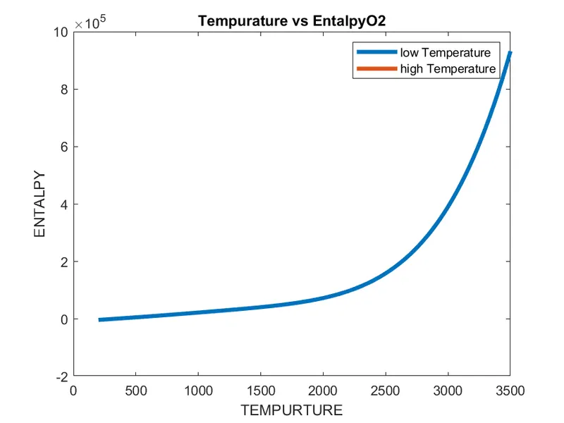
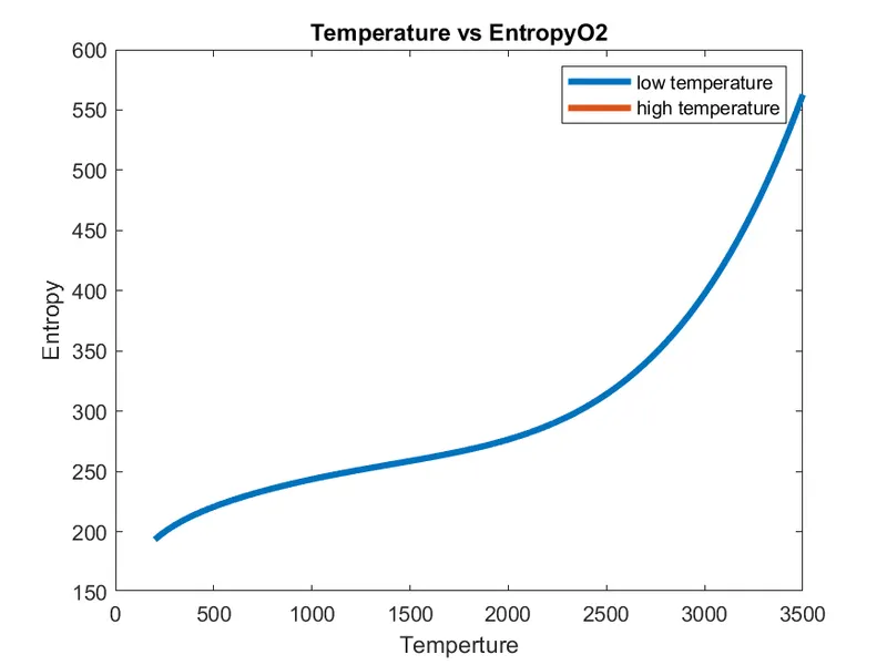
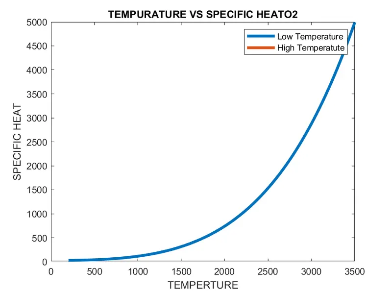
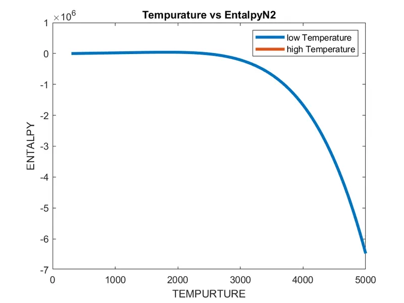
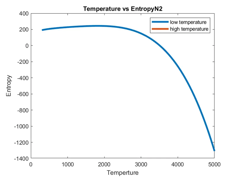
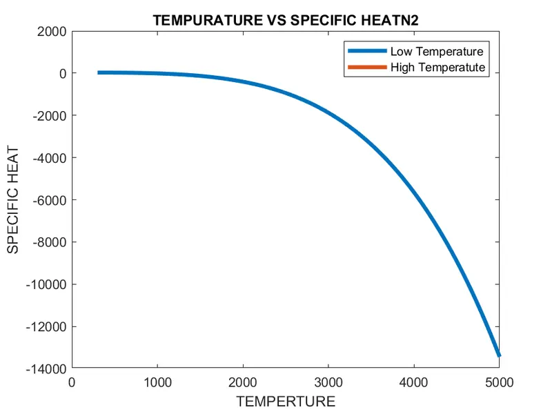
AS SAME AS ABOVE ALL PLOT WE GET THE PLOT OF FILES SHOWN IN FIGURE BELOW AND ALL ARE SAVED AS EACH FILES

THE COMMAND BOX RESULTS ARE