Week 4.1 - Genetic Algorithm
GENETIC ALGORITHM:
genetic algorithm is an optimisation technique to find the maximia and minima using iterative method over the successive iterations the population evolves and get towards the optimal solution
important concepts of optimisation are
1.selection
2.crossover
3.mutation
selection is process in which best performing values in region taken into consideration as they provide better values according to the given function.
crossover is phenomenon where best performing pair of the selection process are taken among the pair. then creating a new set of values by the similar set of values from the consider pair where this new set of values gives us optimal values than considered pair
mutation is technique which avoids the local minima values from the formed new set so that optimization moves in a correct path.
for example if we concider optimization in binary case:
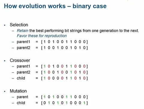
path.
syntax of ga function:
x=ga(fun,nvar,A,b,Aeq,beq,lb,ub,nonlcon,options)
x is the local minima point
fun is the function to be called (stalagmite function)
nvar represents no of variables used
A and b represents the inequalites that exist in the function
Aeq and beq also denotes the inequalities
lb=lower bound
ub= upper bound
noncolon gives a vector representing equalities and inequalities
options is used to perform additional operations such as increasing population size
AIM:
program to calculate the globel minimum using genetic algorithm using MATLAB
GOVERNING EQUATION:
the stalagmate function is as follows
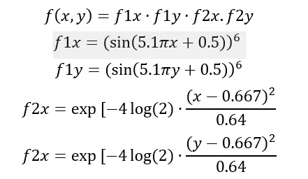
the stalagmate function can be formed using the set of equations provided.this function is helps us to get set of values which inturn helps us to get the three dimensional plot
OBJECTIVES:
the main objective of the project is to find the maxima among the given plot .and provide the set of iterations which in order leads to finding out the maxima
BODY:
programming language used is MATLAB
%stalagmate function in which set of equations are formulated

function [f] = stalagmate(input)

x=input(1);
y=input(2);

f1x=(sin(5.1*pi.*x+0.5)).^6;
f1y=(sin(5.1*pi.*y+0.5)).^6;
f2x=exp(-4*log(2)*(((x-0.0667).^2)./0.64));
f2y=exp(-4*log(2)*(((y-0.0667).^2)./0.64));

f=-f1x*f2x*f1y*f2y;

end
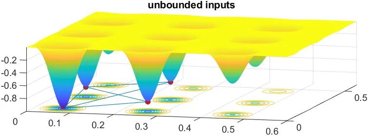
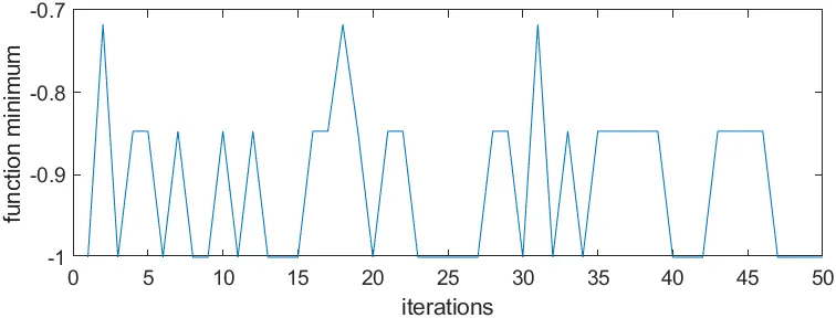
stage1(iteration with out any boundaries):
clear all
close all
clc

%linspace is a command which can takes set of values in between a set of values

x=linspace(0,0.6,150);
y=linspace(0,0.6,150);
num_count=50;

%creating a two dimensional array
% meshgrid command is used to create 2d array

[xx, yy] = meshgrid(x,y);

%evaluating the stalagmate function
%nested for loop  in order to create a space using stalagmate function

for i=1:length(xx)
    for j=1:length(yy)
        input_vector(1)=xx(i,j);
        input_vector(2)=yy(i,j);
        f(i,j)=stalagmate(input_vector);
    end
end

%tic and toc command is used to find the iteration duration
%genetic function is used for the optimization to find the maxima or minima
%of the space

tic

for i=1:num_count
    [input,fopt(i)]=ga(@stalagmate,2)
    xopt(i)=input(1);
    yopt(i)=input(2);

end

%represents the duration of iteration

study_time=toc

figure(1)

%subplot is used represent the part of the 3d plot

subplot(2,1,1);

%surfc command is used to plot the 3d plot

surfc(x,y,f)

%interp command is used to get grid free plot

shading interp

hold on

plot3(xopt,yopt,fopt, 'Marker','o','MarkerSize',5,'MarkerFaceColor','r')
title('unbounded inputs')
subplot(2,1,2)
plot(fopt)
xlabel('iterations')
ylabel('function minimum')
results:
study_time =
1.8756
graph:
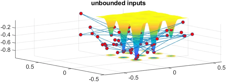
n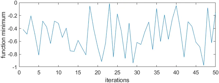
stage2 ( iteration using the bondaries)
close all
clear all
clc
%linspace is a command which can takes set of values in between a set of values
x=linspace(0,0.6,150);
y=linspace(0,0.6,150);
num_count=50;
%creating a two dimensional array
%meshgrid command is used to create 2d array

[xx, yy] = meshgrid(x,y);

%evaluating the stalagmate function
%nested for loop  in order to create a space using stalagmate function


for i=1:length(xx)
    for j=1:length(yy)
        input_vector(1)=xx(i,j);
        input_vector(2)=yy(i,j);
        f(i,j)=stalagmate(input_vector);
    end
end

%tic and toc command is used to find the iteration duration
%genetic function is used for the optimization to find the maxima or minima
%of the space with in the boundaries so that optimization limits to certain
%region

tic

for i=1:num_count
    [input,fopt(i)]=ga(@stalagmate,2,[],[],[],[],[0;0],[1;1])
    xopt(i)=input(1);
    yopt(i)=input(2);

end

%represents the duration of iteration

study_time=toc
figure(2)

%subplot command plot the 1d plot of space

subplot(2,1,1);

%surfc command is used to plot the 3d plot

surfc(x,y,f);

%interp command is used to get grid free plot

shading interp
hold on


plot3(xopt,yopt,fopt, 'Marker','o','MarkerSize',5,'MarkerFaceColor','r')

title('unbounded inputs')
subplot(2,1,2);
plot(fopt);
xlabel('iterations')
ylabel('function minimum')
result:
study_time =
2.8526
graph:
stage3 (iteration with boundaries with increased no of iterations)
close all
clear all
clc
%linspace is a command which can takes set of values in between a set of values
x=linspace(0,0.6,150);
y=linspace(0,0.6,150);
num_count=50;

%creating a two dimensional array
%meshgrid command is used to create 2d array

[xx, yy] = meshgrid(x,y);

%evaluating the stalagmate function
%nested for loop  in order to create a space using stalagmate function


for i=1:length(xx)
    for j=1:length(yy)
        input_vector(1)=xx(i,j);
        input_vector(2)=yy(i,j);
        f(i,j)=stalagmate(input_vector);
    end
end

%tic and toc command is used to find the iteration duration
%genetic function is used for the optimization to find the maxima or minima
%of the space with in the boundaries so that optimization limits to certain
%region

options=optimoptions('ga')
options=optimoptions(options,'PopulationSize',170)
tic
for i=1:num_count
    [input,fopt(i)]=ga(@stalagmate,2,[],[],[],[],[0;0],[1;1],[],[],options)
    xopt(i)=input(1);
    yopt(i)=input(2);

end

%represents the duration of iteration

study_time=toc
figure(2)

%subplot command plot the 1d plot of space

subplot(2,1,1);

%surfc command is used to plot the 3d plot

surfc(x,y,f)

%interp command is used to get grid free plot

shading interp

hold on

plot3(xopt,yopt,fopt, 'Marker','o','MarkerSize',5,'MarkerFaceColor','r')
title('unbounded inputs')
subplot(2,1,2)
plot(fopt)
xlabel('iterations')
ylabel('function minimum')
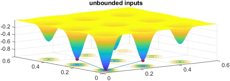
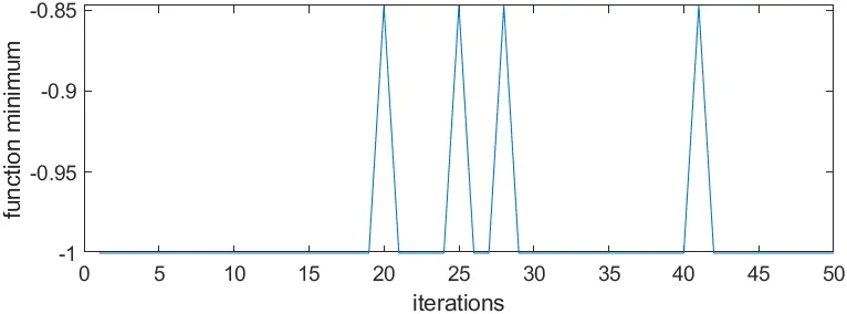
result:
study_time =
5.9871
graph:
CONCLUSION:
optimisation technique is the basic of this project .initilization is first step where we have to assume a set of values which satisfy the function.then evaluation of the algorithm takes place where iterations using the concepts of selection,crossover and mutation takes place which lead us to optimal solution i.e globel maxima
in our project we have concidered three iterations in iteration1 where we are not taken into concideration providing a random samples which is not correct,in the iteration2 we are assumed boundaries so we have samples which are heading in the right path.in the iteration3 along with the boundaries we also assumed increasing the population size which lead to globel minima so as the increasing population size also increases the time of computing