Week 4.1 - Genetic Algorithm

GENETIC ALGORITHM

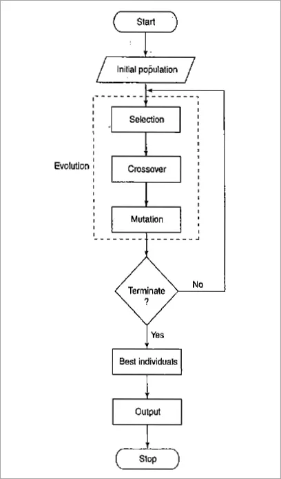
A genetic algorithm is a method for solving both constrained and unconstrained optimization problems based on a natural selection process that mimics biological evolution. The algorithm repeatedly modifies a population of individual solutions. At each step, the genetic algorithm randomly selects individuals from the current population and uses them as parents to produce the children for the next generation. Over successive generations, the population evolves towards an optimal solution.

We can use the genetic algorithm to solve difficulties that are not well suited for standard optimization algorithms, including concerns in which the objective function in discontinuous, non-differentiable, stochastic or highly nonlinear.

In classical algorithm, it generates the single point at each iteration and sequence of points approaches an optimal solution whereas in genetic algorithm it generates the population of points at each iteration and the best point in the population approaches an optimal solution.

Procedure of genetic algorithm

syntax of genetic algorithm in MATLAB

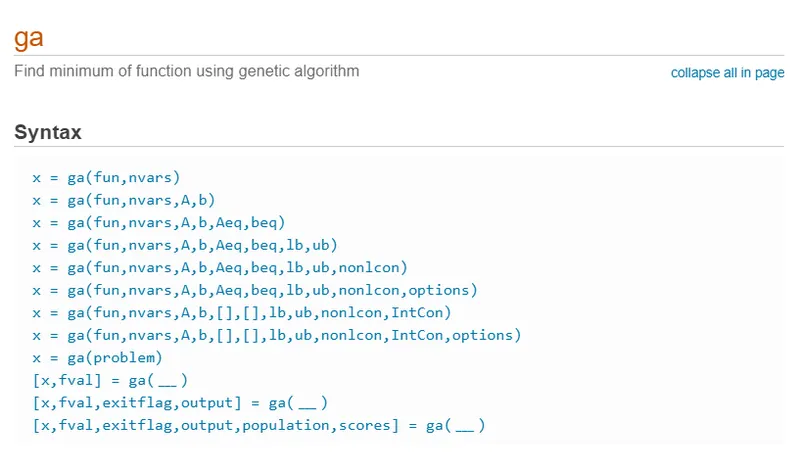
Description

FUNCTION FILE

function [f] = stalagmite(input_vector)

x = input_vector(1);
y = input_vector(2);

f1_x = (sin(5.1*pi*x+0.5))^6;
f1_y = (sin(5.1*pi*y+0.5))^6;

t1 = ((x-0.0667)^2)/(0.64);
f2_x = exp(-4*log(2)*t1);

t2 = ((y-0.0667)^2)/(0.64);
f2_y = exp(-4*log(2)*t2);

f = -(f1_x*f1_y*f2_x*f2_y);

end

Here we created a code to calculate the global maxima and local maxima of a stalagmite function, including the code of a function it was named as stalagmite.

The function consists of 4 different functions which has been evaluated and calculated separately along with their product.

CODE

code for individual global maxima and local maxima

First we need to create a dataset of x and y where the space is represented that where we can perform the genetic algorithm.

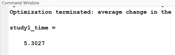
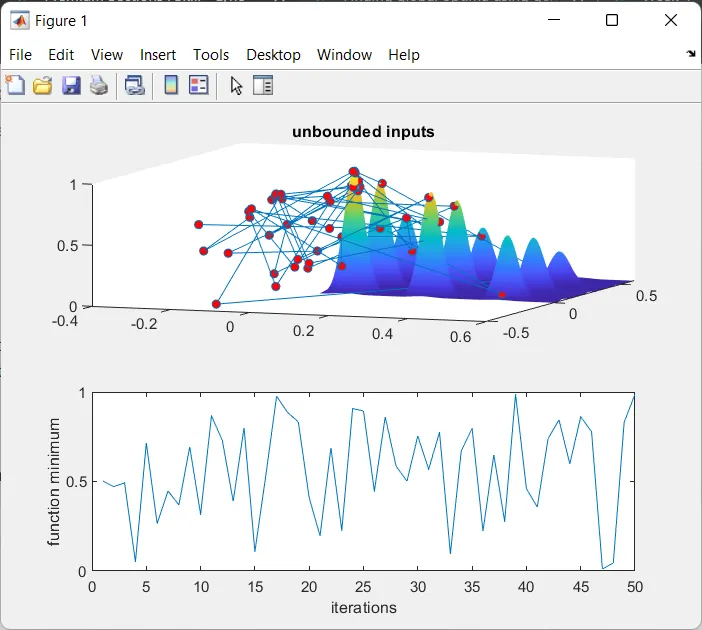
In study 1, we have to study the statistical behavior of the genetic algorithm. We created a for loop where we can use the GA on stalagmite. We have tic and toc operator to calculate the time taken to study. -ve sign is used in plots to create the global maxima.

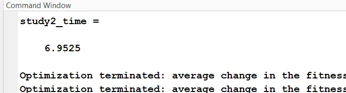
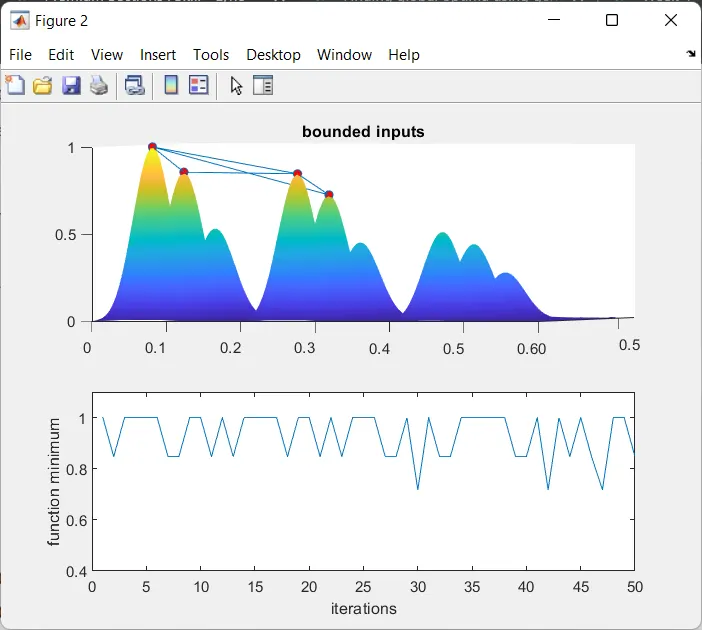
In study 2, we again perform the statistical behavior with upper and lower boundaries. The boundaries help us to improve the optimization of the solution. It shows the better result when compared to the previous one.

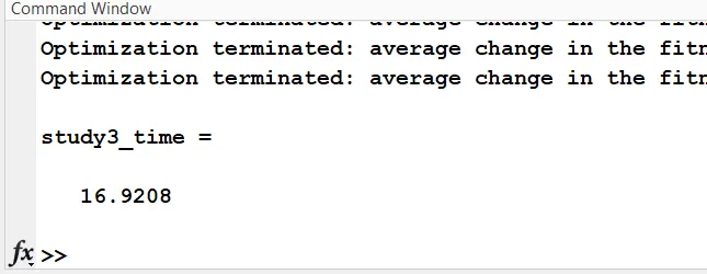
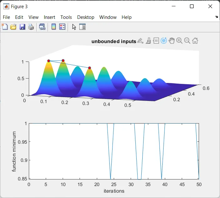
In study 3, We have another constraint used known as Options helps us to increase the population to increase the size. Increasing the iterations helps us to reduce the errors.

clear all
close all
clc

% input variables 
x = linspace(0,0.6,150);
y = linspace(0,0.6,150);

% creating 2D mesh
[xx,yy] = meshgrid(x,y);

for i = 1:length(xx);
    for j = 1:length(yy);
        input_vector(1) = xx(i,j);
        input_vector(2) = yy(i,j);
        f(i,j) = stalagmite(input_vector);
    end
end

surf(xx,yy,-f)
shading interp

[x,fval]=ga(@stalagmite,2)

Output

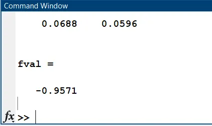
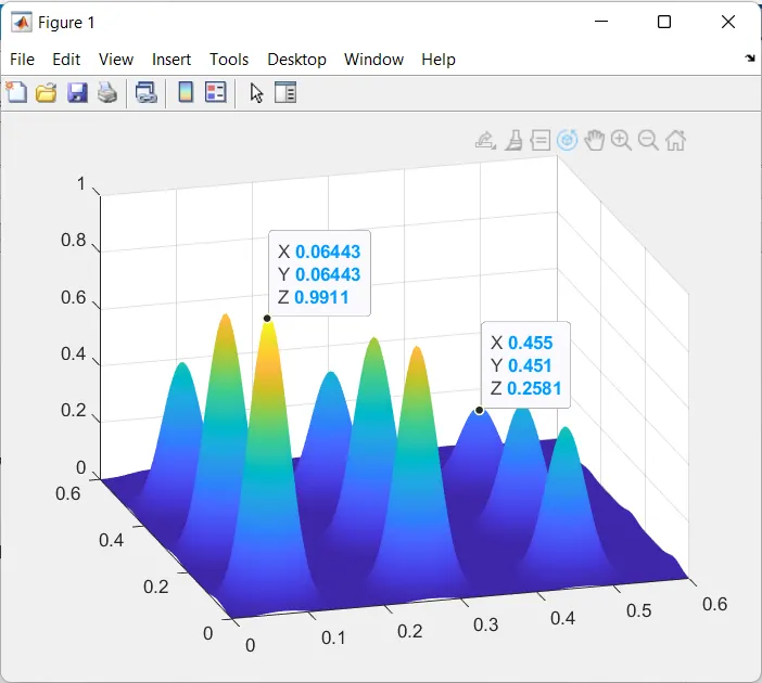
Code for stalagmite function with 3 studies

clear all 
close all
clc

% search space %
x = linspace(0,0.6,150);
y = linspace(0,0.6,150);
num_cases = 50

% 2D mesh %
[xx,yy] = meshgrid(x,y);

% evaluating the stalagmite function %
for i = 1:length(xx);
    for j = 1:length(yy);
        input_vector(1) = xx(i,j);
        input_vector(2) = yy(i,j);
        f(i,j) = stalagmite(input_vector);
    end
end

% =================== study-1 statistical beahviour ===================== %
tic
for i = 1:num_cases;
    [inputs, fopt1(i)] = ga(@stalagmite,2);
    xopt1(i) = inputs(1);
    yopt1(i) = inputs(2);
end

study1_time = toc

figure(1)
subplot(2,1,1)
hold on
surf(x,y,-f)
shading interp
plot3(xopt1,yopt1,-fopt1,'marker','o','markersize',5,'markerfacecolor','r')
title('unbounded inputs')
subplot(2,1,2)
plot(-fopt1)
xlabel('iterations')
ylabel('function minimum')


% ==== study-2 statistical bahaviour - with upper and lower bounds =======%
tic
for i = 1:num_cases;
    [inputs,fopt2(i)] = ga(@stalagmite,2,[],[],[],[],[0;0],[1;1]);
    xopt2(i) = inputs(1);
    yopt2(i) = inputs(2);
end

study2_time = toc

figure(2)
subplot(2,1,1)
hold on
surf(x,y,-f)
shading interp
plot3(xopt2,yopt2,-fopt2,'marker','o','markersize',5,'markerfacecolor','r')
title('bounded inputs')
subplot(2,1,2)
plot(-fopt2)
axis([0 50 0.4 1.1])
xlabel('iterations')
ylabel('function minimum')

% ================= study-3 increasing GA interations ====================%
options = optimoptions('ga');
options = optimoptions(options, 'populationsize',170);

tic
for i = 1:num_cases;
    [inputs,fopt3(i)] = ga(@stalagmite,2,[],[],[],[],[0;0],[1,1],[],[],options);
    xopt3(i) = inputs(1);
    yopt3(i) = inputs(2);
end

study3_time = toc

figure(3)
subplot(2,1,1)
hold on
surf(x,y,-f)
shading interp
plot3(xopt3,yopt3,-fopt3,'marker','o','markersize',5,'markerfacecolor','r')
title('unbounded inputs')
subplot(2,1,2)
plot(-fopt3)
xlabel('iterations')
ylabel('function minimum')

OUTPUTS

study 1

study 2

study 3

Errors

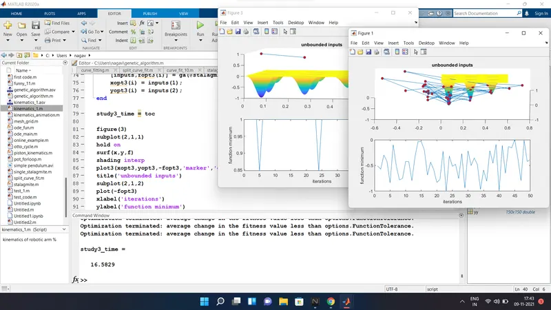
As shown in the above snap, I have faced an error showing that all my regions are reversed. The output gives the results of local minima and global minima. I observed I forgot to place a negative symbol in plots. So the problem can be rectified by pacing a negative symbol in the plots.

THANK YOU