Week 3 - Solving second order ODEs

ODE equation of SIMPLE PENDULUM

The Differential equations have wide applications in various engineering and science disciplines. In general, modeling
of the variation of a physical quantity, such as temperature, pressure, displacement, velocity, stress, strain, current,
voltage, or concentration of a pollutant, with the change of time or location, or both would result in differential
equations. Similarly, studying the variation of some physical quantities on other physical quantities would also lead to
differential equations.

The ODE equation of motion of a simple pendulum with damping factor is written as

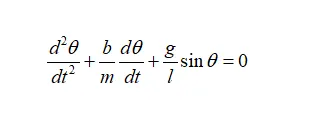
In the above equation,

g = gravity in m/s2

L = length of the pendulum in m

m = mass of the ball in kg

b = damping coefficient

The above given equation having differential power of order 2. In MATLAB, we use 'ode45' solver to solve this second order differential equation. Any order of differential equations are solved using this solver, but we have to give input in a simple differential equation form.

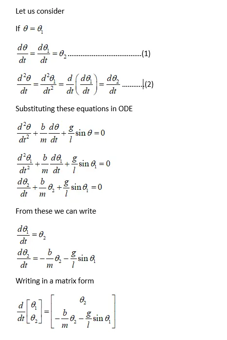
Using this matrix form and ode45 solver, we can create the animation in MATLAB using the following code.

CODE :

close all 
clear all
clc

b = 0.05;
g = 9.81;
l = 1;
m = 1;

% initial condition %
theta_0 = [0;3];

% time points %
t_span = linspace(0,20,500);

% solve ODE %
[t, results] = ode45(@(t,theta) ode_fun(t,theta,b,g,l,m),t_span, theta_0);

% plotting for angular velocity and displacement %
figure(1)
title('motion of pendulum')
plot(t,results(:,1))
hold on
plot(t,results(:,2))
ylabel('angular velocity (rad/s)/ displacement (rad)')
xlabel('time (sec)')
legend('displacement','angular velocity')

angle = results(:,1);

ct = 1
for i = 1:length(angle);
    omega = angle(i);
    
    figure(2)
    % fixed coordinates of one end of pendulum
    x0 = 0;
    y0 = 0;
    % free end coordinates
    x1 = l*cos((3*pi/2)+omega);
    y1 = l*sin((3*pi/2)+omega);
    
    % bob motion
    plot([x0 x1],[y0 y1],'linewidth',3,'color','g')
    hold on
    plot(x1,y1,'O','markers',15,'markerfacecolor','r')
    hold on
    plot([-2 2],[0 0],'linewidth',2,'color','k')
    hold off
    axis([-2 2 -2 2])
    grid on
    pause(0.01)
    M(ct) = getframe(gcf)
    ct = ct+1;
end

% creating video file %
movie(M)
Videofile = VideoWriter('simple pendulum.avi','uncompressed AVI')
open (Videofile)
writeVideo(Videofile,M)
close(Videofile)

CODE EXPLANATION :

• The program is started with the basic commands such as 'close all', 'clear all, 'clc'.
• The input values are specified

length of string (l) = 1 m

mass of bob (m) = 1 Kg

damping coefficient (b) = 0.05

gravity (g) = 9.81 m/s2

• At initial condition when theta is equal to zero, the displacement is zero and the angular velocity is taken 3 rad/sec as given.
• In Ode45 solver, t_span command is used to specify the time span of the simulation. As specified in the given data, it was taken as 0-20 sec. The number of iterations is taken depending upon the smoothness of the output animation. Here I have taken 500 iterations to get a smooth output animation video.
• In the given differential equation, the higher order of degree is two. So we have to take two constants i.e, theta1 and theta2 to simply it into simple differential equation.
• In the syntax of ode45 solver, the function should take at least two inputs to solve the equation, and also we have to specify the t and y.
• In figure 1, the values of the displacement and angular velocity are plotted. Hold on command is used to plot both the angular velocity and displacement.
• To animate the simple pendulum, for loop is used to create the specified set of points to keep the bob at different locations.
• The one end of the string are fixed, i.e., x0 =0 and y0 = 0. The other of the end string which is connected to the bob are found using the trigonometric functions.
• ct command is used to count the every position of the bob.

• An array called 'M' is created, the total resulting frames will be collected in this array. Every time, the current frame resulting from the loop is saved in this array because of the command 'getframe(gcf)' with the counter value always incrementing before the end of the loop.

• Then the animation is made as a video file with file name 'Forward_kinematics.avi'. All frames are gathered and arranged is sequence to create a video file.

ODE FUNCTION CODE :

function [dtheta_dt] = ode_fun(t, theta, b, g, l, m)

theta1 = theta(1);
theta2 = theta(2);

dtheta1_dt = theta2;
dtheta2_dt = -(b/m)*theta2 -(g/l)*sin(theta1);

dtheta_dt = [dtheta1_dt ; dtheta2_dt];

end

• Function file is created which solves the simple differential equation with specified commands. In this function, we have to specify the input values such as time, angle, gravity, damping coefficient, length of string and mass.

OUTPUT :

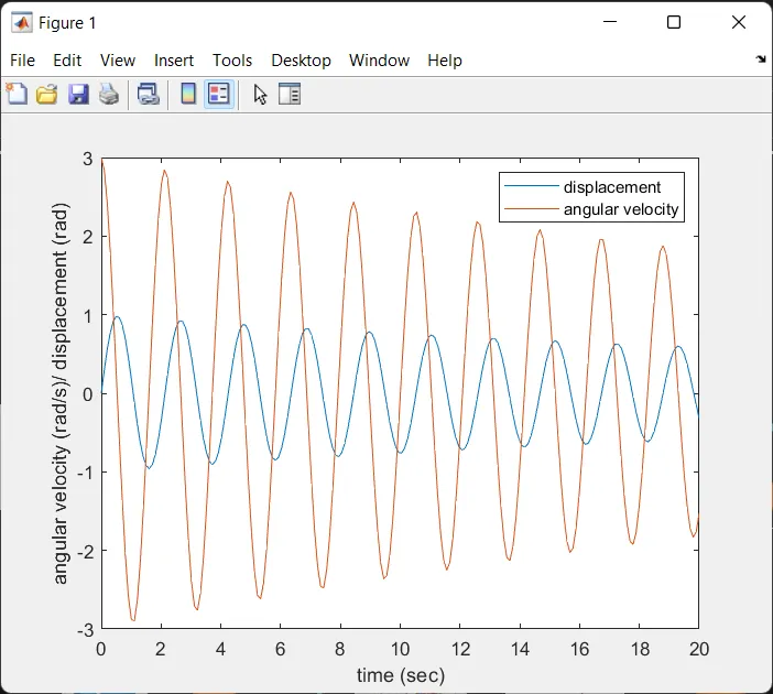
• A plot is created between time and angular velocity/displacement. As mentioned in the given data, the motion of the pendulum is simulated from 0-20 sec.
• The blue plot indicates displacement and the red plot indicates angular velocity.

ANIMATION VIDEO :

The animation video of the simple pendulum

https://youtu.be/3J5CCUfnJqk

ERRORS :

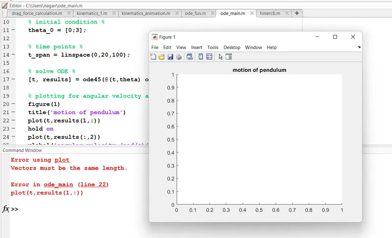
This error I have faced during plotting of figure 1. The inputs are given in the form of the 1X2 matrix, In first column displacement is taken and in second column angular velocity is taken. So the plot is crated between the given time span and 20 seconds and the displacement which has been created. The results of the ode are created in 2X500 matrix form. In this, the first column contains the output values of the angular velocity and the second column contains the output values of displacement in 500 rows because we have taken 500 iterations.

By considering the first column and all rows, the plot between velocity and the time span is created. When we plot between second column and all rows creates the plot between displacement and time.

Initially I faced an error in this and later rectified.

THANK YOU