Project 2 - Rankine cycle Simulator
Rankine Cycle Simulator
The Rankine vapor cycle is a process which is widely used in the power plants, which are coal-fired power plants. In this process, the fuel is used to produce heat within the boiler and this heat is transferred to the medium, usually water. Due to heating of water, it was converted into steam and this steam is then expanded in the turbine to produce useful work.
The basic components of Rankine cycle are :
- Boiler
- Turbine
- Condenser
- Pump
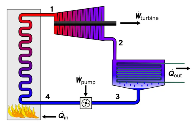
From the above diagram
1-2 process :
Isentropic expansion in the turbine :- In the turbine, the high pressure and temperature steam is expanded isentropically over the turbine blades. The turbine work output is obtained Wt.
2-3 process :
Isobaric heat rejection in condenser :- In condenser, the exhaust gases from the turbine are cooled using external water. The hot steam is condensed into water and then fed to the pump. The heat rejected from the water Qout.
3-4 process :
Isentropic compression in pump :- The condensate from the condenser is again fed into the boiler tube with increased pressure. Work done by the pump Wp.
4-1 process :
Isobaric heat addition in boiler :- The heat is added to the water by firing of coal inside it. Due to addition of heat, the water is gets converted into the steam. Heat added to the water in the boiler, Qin.
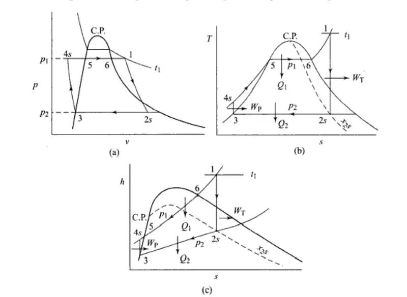
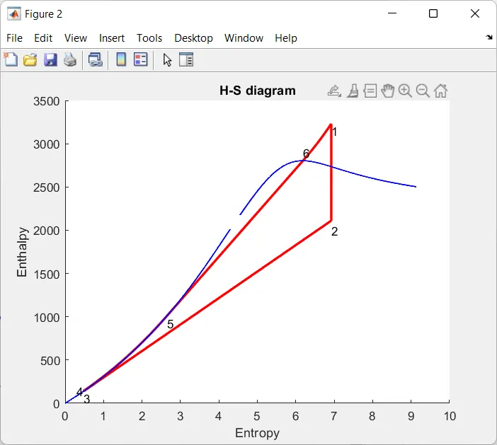
P-V, T-S and H-S diagrams :
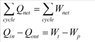
Applying steady state energy equation
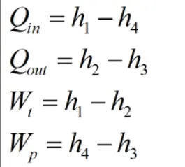
Where
Efficiency of the cycle

We have to find
1. net work output (KJ/Kg)
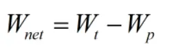
2. Back work ratio
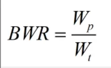
CODE :
% ===================== RANKINE CYCLE SIMULATOR ========================= %
clear all
close all
clc

% ===================== rankine cycle processes ========================= %
fprintf('     RANKINE CYCLE SIMULATOR')
fprintf('\n1-2 Isentropic expansion in Turbine')
fprintf('\n2-3 Isobaric heat rejection by condensor')
fprintf('\n3-4 Isentropic compression in pump')
fprintf('\n4-1 Isobaric heat addition by boiler \n')
fprintf('\n')

% Given inputs %
P1 = input('pressure at turbine inlet (bar)        :');
T1 = input('temperature at turbine inlet (celsius) :');
P2 = input('pressure at condensor (bar)            :');

% ==================== Stage -1 (Turbine inlet) ========================= %
% pressure and temperatures are given %
h1 = XSteam('h_pT',P1,T1);
s1 = XSteam('s_pT',P1,T1);

% =================== Stage - 2 (Condenser inlet) ======================= %
% P2 is given % to find h2 %
% h2 = hf2 + x2 (hg2 - hf2) %
% Where x2 = (s2 - sf2)/(sg2 - sf2) %
s2 = s1 ;  % Isentropic process
sf2 = XSteam('sL_p',P2);
sg2 = XSteam('sV_p',P2);
x2 = (s2-sf2)/(sg2-sf2);
hf2 = XSteam('hL_p',P2);
hg2 = XSteam('hV_p',P2);
h2 = hf2 + (x2*(hg2 - hf2));

% ======================= Stage - 3 (Pump inlet) ======================== %
P3 = P2;   % Isobaric process
% saturated liquid stage %
h3 = XSteam('hL_p',P3);
s3 = XSteam('sL_p',P3);
T3 = XSteam('Tsat_p',P3);
T2 = T3; % for stage - 2

% ======================= Stage - 4 (Boiler inlet)======================= %
s4 = s3; % Isentropic process
P4 = P1; % Isobaric process
h4 = XSteam('h_ps',P4,s4);
% to find T4 % T3/T4 = (P3/P4)^((C-1)/C) %
% Where C = Cp4/Cv4
% Specific heat values %
Cp4 = XSteam('Cp_ps',P4,s4); % constant pressure %
Cv4 = XSteam('Cv_ps',P4,s4); % constant volume %
C = Cp4/Cv4;
T4 = T3/((P3/P4)^((C-1)/C));

% saturated liquid state %
T5 = XSteam('Tsat_p',P1);
s5 = XSteam('sL_p',P1);
h5 = XSteam('hL_p',P1);

% saturated vapour state %
T6 = T5;
s6 = XSteam('sV_p',P1);
h6 = XSteam('hV_p',P1);

% Calculation of work (KJ/Kg) %
Wt = h1 - h2; % Turbine work
Wp = h4 - h3; % Pump work
W = Wt - Wp;  % Net work Output

% Calculation of heats %
Qin = h1 - h4; % heat addition in boiler
Qout = h2 - h3; % heat removed in condeser

% Thermal Efficiency (%) %
nTherm = (W/Qin)*100;

% Steam rate (Kg/KWh) %
SSC =3600/W;

% Back work ratio %
BWR = Wp/Wt;

% ============================== Plotting =============================== %

% plotting T-S diagram %
figure(1)
hold on
title('T-S diagram')
plot([s1 s2],[T1 T2],'linewidth',2,'color','r')
plot([s2 s3],[T2 T3],'linewidth',2,'color','r')
plot([s3 s4],[T3 T4],'linewidth',2,'color','r')
plot([s4 s5],[T4 T5],'linewidth',2,'color','r')
plot([s5 s6],[T5 T6],'linewidth',2,'color','r')

s_1 = linspace(s6,s1,500);
for j = 1:length(s_1);
    t_1(j) = XSteam('T_ps',P1,s_1(j));
end
plot(s_1,t_1,'linewidth',2,'color','r')
xlabel('Entropy')
ylabel('Temperature')

% plot saturation curve %
T = linspace(1,T1,500);
for i = 1:length(T);
    h_l(i) = XSteam('hL_T',T(i));
    h_v(i) = XSteam('hV_T',T(i));
    s_l(i) = XSteam('sL_T',T(i));
    s_v(i) = XSteam('sV_T',T(i));
end
plot(s_l,T,'linewidth',1,'color','b')
plot(s_v,T,'linewidth',1,'color','b')

% annotations %
text(s1,T1,'1','verticalalignment','top')
text(s2,T2,'2','verticalalignment','cap')
text(s3,T3,'3','verticalalignment','cap')
text(s4,T4,'4','horizontalalignment','right')
text(s5,T5,'5','verticalalignment','top')
text(s6,T6,'6','horizontalalignment','left')

% plotting H-S diagram %
figure(2)
hold on
title('H-S diagram')
plot([s1 s2],[h1 h2],'linewidth',2,'color','r')
plot([s2 s3],[h2 h3],'linewidth',2,'color','r')
plot([s3 s4],[h3 h4],'linewidth',2,'color','r')

h_4 = linspace(h4,h5,500);
for k = 1:length(h_4)
    s_4(k) = XSteam('s_ph',P1,h_4(k));
end

h_6 = linspace(h6,h1,500);
for m = 1:length(h_6)
    s_6(m) = XSteam('s_ph',P1,h_6(m));
end

plot(s_4,h_4,'linewidth',2,'color','r')
plot([s5 s6],[h5 h6],'linewidth',2,'color','r')
plot(s_6,h_6,'linewidth',2,'color','r')
xlabel('Entropy')
ylabel('Enthalpy')

% plot saturation curve %
plot(s_l,h_l,'linewidth',1,'color','b')
plot(s_v,h_v,'linewidth',1,'color','b')

% annotations %
text(s1,h1,'1','verticalalignment','top')
text(s2,h2,'2','verticalalignment','cap')
text(s3,h3,'3','verticalalignment','top')
text(s4,h4,'4','horizontalalignment','right')
text(s5,h5,'5','verticalalignment','top')
text(s6,h6,'6','verticalalignment','bottom')

% Results window %
fprintf('\n     RESULTS')
fprintf('\n >>>At state point 1 :')
fprintf('\n P1 is : %f Bar',P1)
fprintf('\n T1 is : %f Deg celcius',T1)
fprintf('\n H1 is : %f KJ/Kg',h1)
fprintf('\n S1 is : %f KJ/KgK',s1)
fprintf('\n')
fprintf('\n >>>At state point 2 :')
fprintf('\n P2 is : %f Bar',P2)
fprintf('\n T2 is : %f Deg celcius',T2)
fprintf('\n H2 is : %f KJ/Kg',h2)
fprintf('\n S2 is : %f KJ/KgK',s2)
fprintf('\n')
fprintf('\n >>>At state point 3 :')
fprintf('\n P3 is : %f Bar',P3)
fprintf('\n T3 is : %f Deg celcius',T3)
fprintf('\n H3 is : %f KJ/Kg',h3)
fprintf('\n S3 is : %f KJ/KgK',s3)
fprintf('\n')
fprintf('\n >>>At state point 4 :')
fprintf('\n P4 is : %f Bar',P4)
fprintf('\n T4 is : %f Deg celcius',T4)
fprintf('\n H4 is : %f KJ/Kg',h4)
fprintf('\n S4 is : %f KJ/KgK',s4)
fprintf('\n')
fprintf('\n Turbine work       : %f KJ/Kg',Wt)
fprintf('\n Pump work          : %f KJ/Kg',Wp)
fprintf('\n Net work output    : %f KJ/Kg',W)
fprintf('\n Thermal efficiency : %f percent',nTherm)
fprintf('\n SSC                : %f Kg/KWh',SSC)
fprintf('\n Back work ratio    : %f',BWR)
fprintf('\n')
Code explanation :
- The program is started with the clear all, close all and clc to clear the workspace, command window and plots.
- Information about the cycle and their processes are mentioned using the 'fprintf' command.
- Input variables P1, T1 and P2 are given by 'input' command whose values are entered in command window while executing the program.
- The data for the properties of steam and water are extracted from the XSteam.m file.
- At state 1, the values for the enthalpy and entropy are extracted as a function of temperature and pressure.
- Similarly, at all states are extracted.
- The formula for calculating the unknown state values of temperature, pressure, enthalpy and entropy are calculated from the basic formulas from reference book.
- After calculating the values at all states, work done and heat transfer are calculated.
- The efficiency, specific steam consumption and back work ratio are also calculate using the above formulas.
- The saturation curve is plotted, temperature range is defined using the 'linspace' command and values of enthalpy and entropy are calculated at each temperature point. These values are used to draw the saturation curves in the h-s and t-s diagrams.
- Now the cycle is plotted over the saturation curve and annotations for each process are specified using the 'text' command.
- All the results of the Rankine cycle are plotted using the 'fprintf' command.
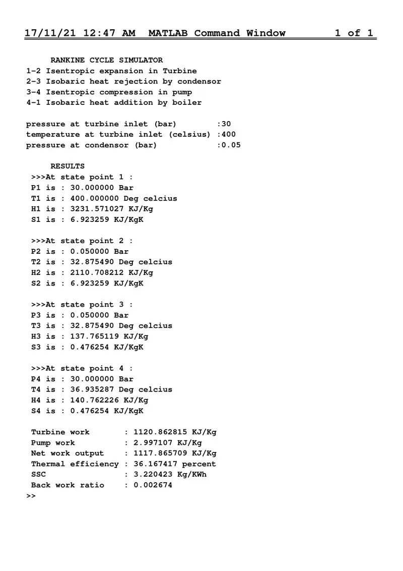
RESULTS :
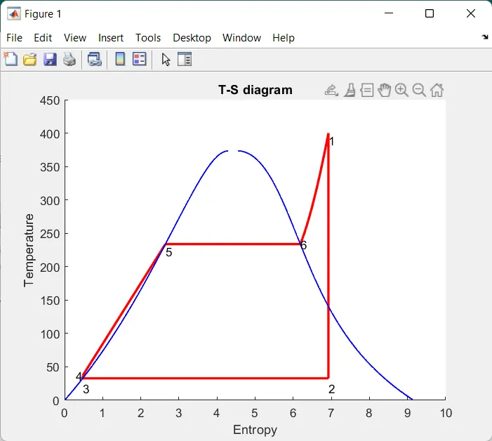
PLOTS :
ERRORS :
Some typo errors are occurred, and later I rectified them.
CONCLUSION :
The values of net work and back work ratio of the Rankine cycle are obtained and t-s and h-s diagrams are plotted.
THANK YOU
References
https://thermopedia.com/content/1072
http://www.ecourses.ou.edu/cgi-bin/ebook.cgi?topic=th&chap_sec=10.1&page=theory
Power Plant Engineering by P K Nag