Week 4.1 - Genetic Algorithm

Objective: To write a code to optimize the stalagmite function and find the global maxima of the function.

Theory: Genetic Algorithm(GA) is a special case of Evolutionary algorithm(EA) which was proposed by charles darwin. A genetic algorithm (GA) is a method for solving both constrained and unconstrained optimization problems based on a natural selection process that mimics biological evolution. The algorithm repeatedly modifies a population of individual solutions. At each step, the genetic algorithm randomly selects individuals from the current population and uses them as parents to produce the children for the next generation. Over successive generations, the population "evolves" toward an optimal solution. It provides efficient and effective techniques for optimization and machine learning application used to create high quality solutions to optimization problems. Widely used in bussiness, scientific and engineering circles.

Stalagmite function : is a mathematical model that helps to generate maximas and minimas.Global maxima is a maximum peak value in entire function and global minima is a minimum peak value in entire function. But local maxima and local minima are multiple number of values.

The following outline summarizes how the genetic algorithm works:

• The algorithm begins by creating a random initial population .
• The algorithm then creates a sequence of new populations .
• At each step, the algorithm uses the individuals in the current generation to create the next population.

• To create the new population, the algorithm performs the following steps:

  1. Scores each member of the current population by computing its fitness value. These values are called the raw fitness scores.

  2. Scales the raw fitness scores to convert them into a more usable range of values. These scaled values are called expectation values.

  3. Selects members, called parents, based on their expectation.

  4. Some of the individuals in the current population that have lower fitness are chosen as elite. These elite individuals are passed to the next population.

  5. Produces children from the parents. Children are produced either by making random changes to a single parent—mutation—or by combining the vector entries of a pair of parents—crossover.

  6. Replaces the current population with the children to form the next generation.

• The algorithm stops when one of the stopping criteria is met.

Stopping Conditions for the Algorithm

The genetic algorithm uses the following options to determine when to stop.

The algorithm stops as soon as any one of these conditions is met.

General syntax for genetic algorithm

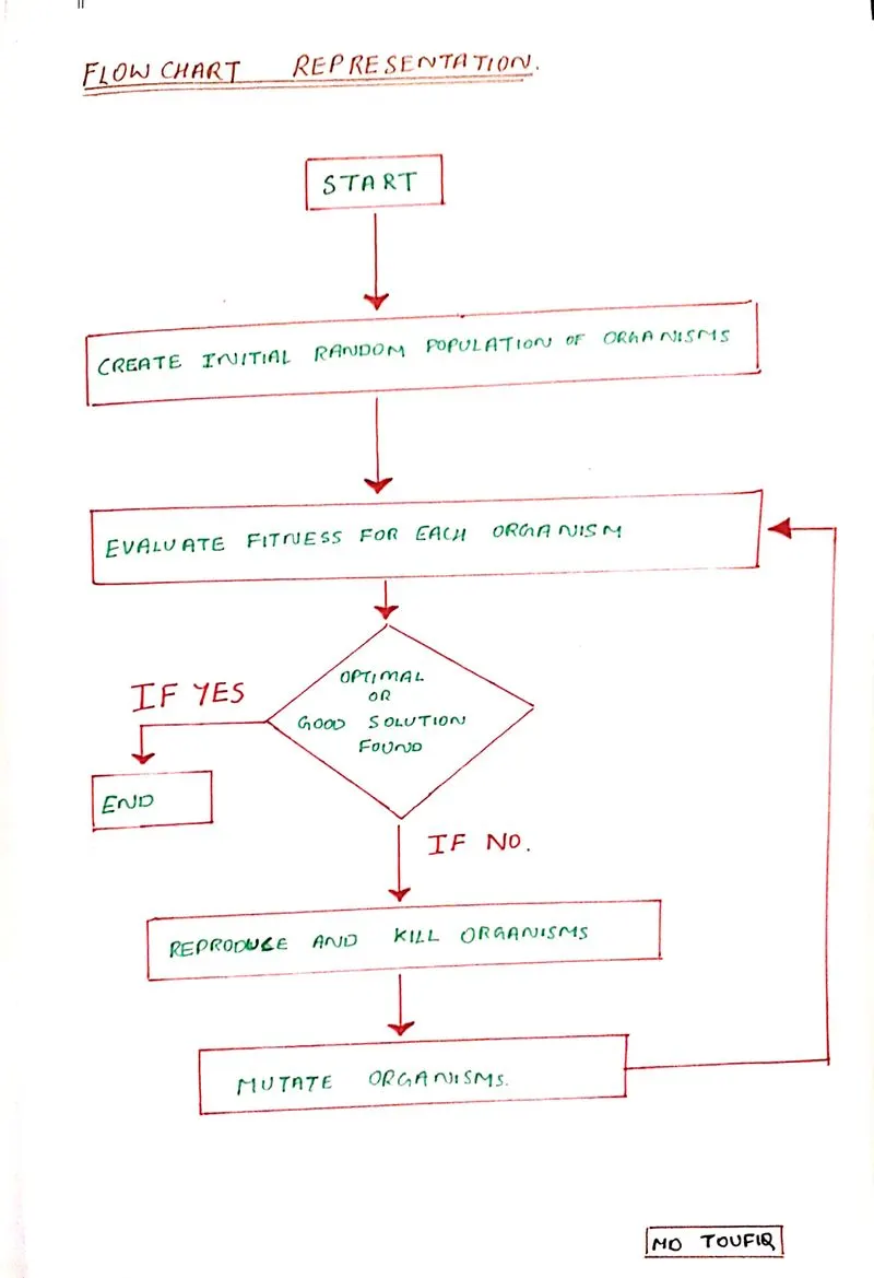
The pictures below show the steps involved and flowchart for Genetic Algorithm.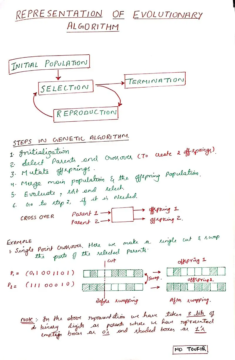

 1.Explanation of the code.

Starting with initializing and declaring range of x-values and y-values and 200 divisions between them and also the value for number of iterations. Later on creating a mesh using the x and y values.

Evaluating the stalagmite function: using first for loop we access all 200 x-values and using second for loop accessing all 200 y-values. When usin stalagmite function we have to assign two variables separately to assign the points of the meshgrid so we are using input_vector(1) and input_vector(2) and then calling the stalgmite function to calcaluate the function for which a separate code is written as per the formulas given and storing the value in f(i,j).

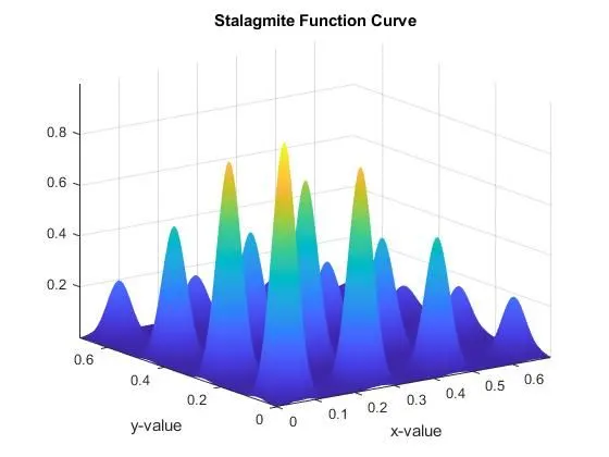
After that creating a plot of stalgmite function which shows a series of maximas and minimas 

using the label command labelling the x and y axis.

shading interp is a command used to hide the grid on the surface of stalagmite plot

After that we are going to make 3 different studies namely:-

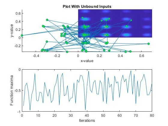
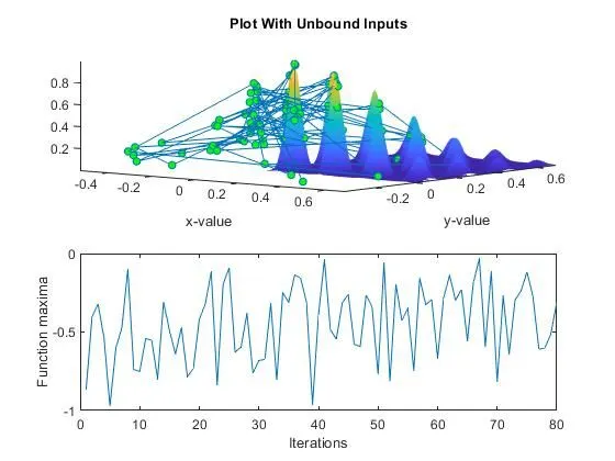
1.statistical behaviour for unbound curve: In this case we are going the use ga(genetic algorithm) inbuilt function to calculate the optimum( minimum) value of the given stalagmite function and evaluating the point where the minima is present but without specifying any bounds. The time taken to run is also calculated and the plot is obtained here plot3 command is used to obtain a 3d plot and also we are using a subplot command to obtain 2 plots in the same window.

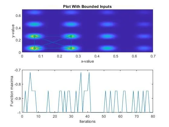
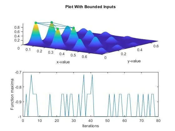
2.statistical behaviour with upper and lower bound: In this case we are following the same procedure as the 1st case but in addition to that we are specifying the boundaries to overcome the problem of getting multiple optimum values as in the 1st case.

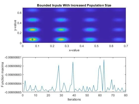
3.statistical behavior by increasing the population size: here also we are going to follow the same procedure as in the second case with bounds but in addition to that we using options function to increase the population size and then evaluating the result and in this case we get a single optimum values no matter how many time we run the code.

clear all
close all
clc

%defining search space
x=linspace(0,0.7,200);      %Splitting x values into 200 divisions
y=linspace(0,0.7,200);      %Splitting y values into 200 divisions
num_case = 80;         %Runnig genetic algorithm 80 times to test the precision of ga.

%creating 2d mesh
[A, B] = meshgrid(x,y);

%Evaluating stalagmite function.
for i = 1:length(A)        %creating for loop to access all 200 values for x-axis.
    for j = 1:length(B)    %creating for loop to access all 200 values for y-axis.
        input_vector(1) = A(i,j);  %for stalagmite we have to separately assign input varibles 
        input_vector(2) = B(i,j);  %for stalagmite we have to separately assign input 
                                               varibles
        f(i,j) = stalagmite(input_vector);    %Function call statement to calculate 
                                                 stalagmite funtion.
    end
end

figure(1)          %creating figure 
surfc(A,B,-f)      %creating a surface for the stalagmite function 
xlabel('xvalue')   %labelling x-axis
ylabel('yvalue')   %labelling y-axis
shading interp     %To hide the grid lines on the surface and make the curve smooth


%Study_1 statistical behavior for unbound curve
tic
for i = 1:num_case
    [inputs1, fopt1(i)] = ga(@stalagmite, 2); %Calculating optimum value(minima or 
                   maxima) using inbuilt ga function for the stalagmite function and 
                   getting the optimum or minima value(fopt) and the point where the 
                   minima is present(inputs1)
    xopt1(i) = inputs1(1); %Assigning the point of minima  in variable xopt.
    yopt1(i) = inputs1(2); %Assigning the point of minima in variable yopt.
end

study_time_1 = toc;     %Calculating the time taken to run.
figure(2)               %Creating figure
subplot(2,1,1)          %Creating subplot(here 2 indicates figure window is divided 
                        into 2 parts to obtain 2 plots in same window)
hold on
surfc(A,B,-f);          %Creating surface using the calculated ga values 
shading interp
plot3(xopt1, yopt1, -fopt1,'marker','o','markersize',5,'markerfacecolor','g'); %Plot3 
                                     command is used to create 3d plot 
title('unbound inputs')              %Giving a title to the plot 
subplot(2,1,2)               %creating subplot to see the variation of optimum value.
plot(fopt1)                  %Plotting the optimum value.
xlabel('iterations')         %labelling x-axis.
ylabel('function maxima')    %labelling y-axis.
 


%study2_statistical behaviour with upper and lower bound
tic                          %Calculating the time taken for the study.
    for i = 1:num_case
    [inputs2, fopt2(i)] = ga(@stalagmite,2,[],[],[],[],[0;0],[0.7;0.7]);  %Calculating 
        optimum value(minima or maxima) using inbuilt ga function for the stalagmite 
        function with the bounds and getting the optimum or minima value(fopt) and the 
        point where the 
     minima is present(inputs1
    xopt2(i) = inputs2(1);    %assigning the point of minima  in variable xopt
    yopt2(i) = inputs2(2);    %assigning the point of minima in variable yopt.
end

study_time_2 = toc
figure(3)                     %Creating figure
subplot(2,1,1)                %creating subplot to see the variation of optimum value.
hold on
surfc(A,B,-f);                %Creating surface using the calculated ga values 
shading interp
plot3(xopt2,yopt2,-fopt2,'marker','o','markersize',5,'markerfacecolor','g')%Plot3 
                                                  command is used to create 3d plot
title('bounded inputs')       %Giving a title to the plot
subplot(2,1,2)
plot(fopt2)
xlabel('iterations')          %labelling x-axis.
ylabel('function maxima')     %labelling y-axis.

%study3_statistical behaviour increasing the ga iterations
tic

options = optimoptions("ga",'populationsize',400); %To increase the number of 
                                                    populations(here 400)
for i = 1:num_case
    [inputs3, fopt3(i)] = ga(@stalagmite,2,[],[],[],[],[0;0],[0.7;0.7],[],[],options); 
      %Calculating optimum value(minima or maxima) using inbuilt ga function for the 
      stalagmite function with the bounds and increased population and getting the 
      optimum or minima value(fopt) and the point where the minima is present(inputs1).
    xopt3(i) = inputs3(1);    %assigning the point of minima  in variable xopt
    yopt3(i) = inputs3(2);    %assigning the point of minima in variable yopt.
end

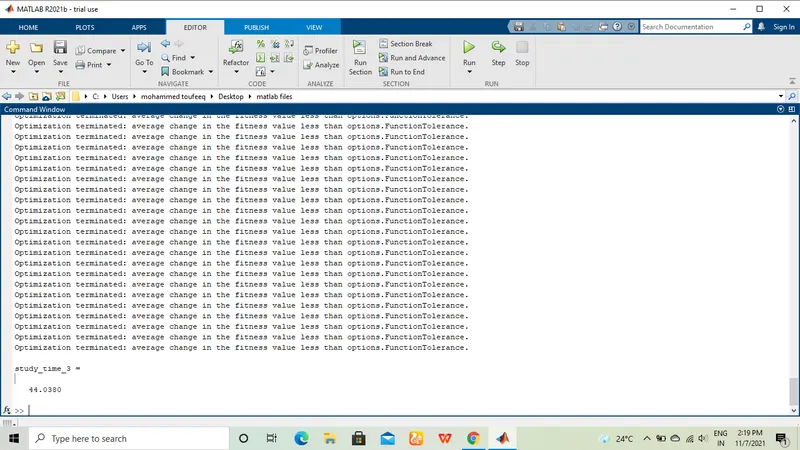
study_time_3 = toc
figure(4)                     %Creating figure
subplot(2,1,1)                %creating subplot to see the variation of optimum value.
hold on
surfc(A,B,-f);                %Creating surface using the calculated ga values 
shading interp
plot3(xopt3,yopt3,-fopt3,'marker','o','markersize',5,'markerfacecolor','g');  %Plot3 
                                    command is used to create 3d plot
title('bounded inputs with increased population size');  %Giving a title to the plot
subplot(2,1,2)
plot(fopt3)                   %Plotting optimum value.
xlabel('iterations')          %labelling x-axis.
ylabel('function maxima')     %labelling y-axis.

Function call (stalagmite function)

function f_xy = stalagmite(input_vector)
x= input_vector(1);    %Assigning the input_vector(1) to variable x.
y = input_vector(2);   %Assigning the input_vector(2) to variable y.
f_1x = (sin((5.1*pi*x)+0.5))^6;  %Calculating the function f1,x as per the given formula 
f_2x = exp(-4*log(2)*(((x-0.0667)^2)/0.64));  %Calculating the function f2,x as per the 
                                              given formula 
f_1y = (sin((5.1*pi*y)+0.5))^6;  %Calculating the function f1,y as per the given formula 
f_2y = exp(-4*log(2)*(((y-0.0667)^2)/0.64));  %Calculating the function f2,y as per the 
                                              given formula 
f_xy = f_1x*f_1y*f_2x*f_2y;    %Calculating the function fxy as per the given formula 
f_xy = -f_xy;     %Negetive sign because the ga calculates only minima. 
end

Results Obtained.

Plot1.

plot2.

plot3

plot4.

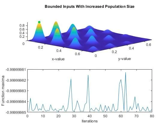
Outputs obtained after succesful running of the code

2.Errors faced while programming

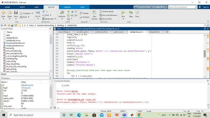
The following error appeared "vectors must of same length" in the line 39 as shown in the screenshot below

Steps taken to overcome the errors.

The above mentioned error appeared because as shown in the screenshot, in workspace there are different values for i (70) and j(200) that is because in the 2nd case of the code, in the for loop part i mistakenly wrote yopt(j) instead of yopt(i) which was taken care off after realizing the error.

References: 1. https://skill-lync.com/student-projects/optimizing-a-stalagmite-function-32889

                    2. https://en.wikipedia.org/wiki/Genetic_algorithm

                    3. https://www.geeksforgeeks.org/genetic-algorithms/

                    4. mathworks.com