Project 2 - Rankine cycle Simulator
AIM : To write a code to create a Rankine Cycle Simulator using Matlab.
OBJECTIVES
- To calculate the state points of the Rankine Cycle (any type of your choice) based on user inputs.
- To plot the corresponding T-s and h-s plots for the given set of inputs.
- To calculate Back work ratio and Net work output.
THEORY
The Rankine cycle or Rankine Vapor Cycle is the process widely used by power plants such as coal fired power plant or nuclear reactors. In this mechanism, a fuel is used to produce heat within a boiler, converting water into steam which then expands through a turbine producing useful work. This process was developed in 1859 by Scottish engineer William J.M. Rankine. This is a thermodynamic cycle which converts heat into mechanical energy which usually gets transformed into electricity by electrical generators.
The Rankine cycle is an idealized thermodynamic cycle describing the process by which certain heat engines, such as steam turbines or reciprocating steam engines, allow mechanical work to be extracted from a fluid as it moves between a heat source and heat sink.
Figure 1. A simple schematic with components for the Rankine Cycle.
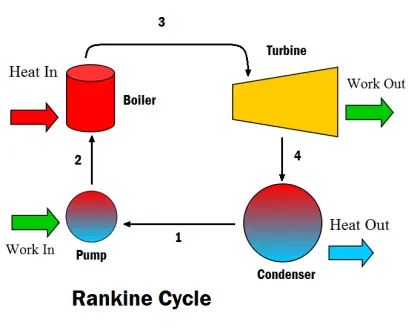
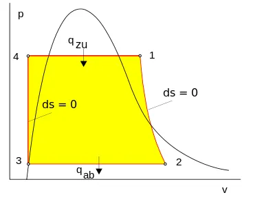
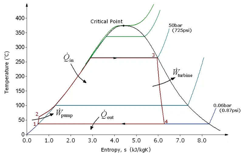
The steps in the Rankine Cycle are as shown in Figure 1 and the corresponding steps in the pressure volume diagram (figure 2) are outlined below:
- Pump: Compression of the fluid to high pressure using a pump (this takes work) (Figure 2: Steps 3 to 4)
- Boiler: The compressed fluid is heated to the final temperature (which is at boiling point), therefore, a phase change occurs—from liquid to vapor. (Figure 2: Steps 4 to 1)
- Turbine: Expansion of the vapor in the turbine. (Figure 2: Steps 1 to 2)
- Condenser: Condensation of the vapor in the condenser (where the waste heat goes to the final heat sink (the atmosphere or a large body of water (ex. lake or river). (Figure 2: Steps 2 to 3)
Equations of Rankine cycle as per the above shown T-s diagram.
1.Pump work, WPumps = H2 – H1.
2.Turbine work, WT = H3– H4.
3. Heat rejection, Qre = H4 – H1.
4. Heat addition, Qadd = H3 – H2.
5.Thermal Efficiency, efficiency = (net work output)/(heat supplied)
.
6.Specific Steam Consumption, 3600/W_net.
7.Back work ratio, bwr = (pump work)/(turbine work).
1.Explanation of the code.
Starting the code by printing the four processes involved in the rankine cycle. And then using the function 'input()' getting the inputs (P1,P2 and T1) from the user.
Next step is to obtain the Thermodynamic properties (i.e specific enthalpy and specific entropy) at state point 1 from the given 'XSteam' file using the predifined functions and the nomenclature provided in the file to calculate the properties as a fucntion of (Temperature, pressure ..etc).
Similarly calculating the thermodynamic properties at state point 2 , 3 and 4, as per the concept of Rankine Cycle and T-s curve.
Later on writing the code to calculate the Turbine work, Pump work, Thermal efficiency, Net work , heat supplied and Specific Steam consumption as per the formulae.
Also calculating the thermodynamic properties at state point 5 and 6 as well to plot the T_s and h-s curve.
And then using the function 'fprintf' to display all the properties at all four state points in the command window and also to display Turbine work(wt), Pump work(wp), Thermal efficiency(effy), Net work(w_net) , heat supplied(Qs) and Specific Steam consumption(steam_rate).
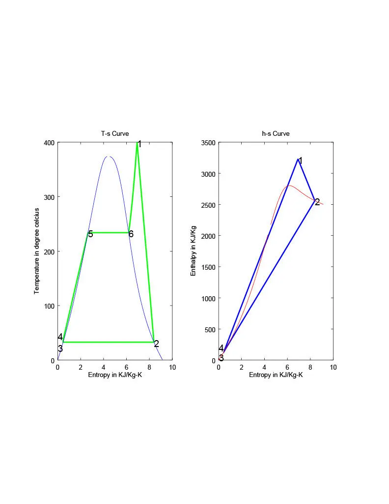
Finally Plotting the T-s and h-s curves. Using the the command 'subplot' to obtain both the plots in the same figure window. Then using Linspace to create 5000 values between the temperatures T5 and T1. Using for loop calculating the corresponding 5000 entropy values for the temperature values.
Later, using the command 'plot' to create T-s curve. And using the function 'text' to give numbers at the state points in the T-s curve. Also using the xlabel and ylabel to label the x-axis and y-axis with appropriate names.
Repeaiting the same procedure to plot the h-s curve as well.
clear all
close all
clc

%The 4 process involved in the cycle.
fprintf(' 1-2 is isentropic expansion process in the turbine.\n')
fprintf(' 2-3 is constant pressure heat rejection in the condensor.\n')
fprintf(' 3-4 is isentropic compression in the pump.\n')
fprintf(' 4-1 is constant pressure heat addition in the boiler.\n\n')

%Getting the inputs from the user
p1 = input('Enter the pressure (in bar) at the inlet of the turbine :')
T1 = input('Enter the temperature (in degree celcius)at the inlet of the turbine :')
p2 = input('Enter the pressure (in bar) at the exit to the turbine :')

%Calculating the thermodynamic properties of steam at state 1 (inlet to the turbine).
h1 = XSteam('h_pT',p1,T1);  %obtaining the enthalpy as a function of pressure and
                            temperature at state 1.
s1 = XSteam('s_pT',p1,T1);  %obtaining the entropy as a function of pressure and
                            temperature at state 1
%Calculating the thermodynamic properties of steam(wet region) at state 2.
s2 = s1;                    %since the process 1-2 is isentropic (i.e entropy remains
                            constant during this process).
sf2 = XSteam('sL_p',p2);    %entropy of liquid phase as a function of pressure
sg2 = XSteam('sV_p',p2);    %entropy of  vapour phase as a function of pressure
hf2 = XSteam('hL_p',p2);    %enthalpy of liquid phase as a function of pressure
hg2 = XSteam('hV_p',p2);    %enthalpy of  vapour phase as a function of pressure
% In wet region, s2 = sf2+x2*sfg => x2 = (s2-sf2)/(sg2-sf2). also sfg = (sg-sf)
s2 = sg2;                   %since the state point 2 lies on the saturated vapour line.
h2 = hg2;                   %since the state point 2 lies on the saturated vapour line.
T2 = XSteam('T_hs',h2,s2);  %obtaining temperature at state point 2 using enthalpy and
                            entropy.

%Calculating the thermodynamic properties of steam at state 3.
T3 = T2;           %from T-S curve ( Temperature remians constant during this process).
p3 = p2;                    %Because 2-3 is a constant pressure process.
s3 = XSteam('sL_T',T3);     %entropy of liquid phase as a function of temperature.
h3 = XSteam('hL_T',T3);     %enthalpy of liquid phase as a function of temperature.
v3 = XSteam('vL_p',p2);     %specific volume of liquid as a function of temperature
%Calculating the thermodynamic properties of steam at state 4.
p4 = p1;                    %since the process 4-1 is a constant pressure process.
s4 = s3;                    %since the process 1-2 is isentropic (i.e entropy remains constant during this process).
cp4 = XSteam('cp_ps',p4,s4);%specific heat at state point 4
cv4 = XSteam('cv_ps',p4,s4);%specific heat at state point 4
gamma = cp4/cv4;            %ratio of specific heats.
r = (gamma-1)/gamma;        %for simplification purpose.
T4 = T3*(p4/p3)^r;          %(T4/T3) = (p4/p3)^(gamma-1)/gamma.
%Calculating other output values.
wt = h1-h2;                 %workdone by the turbine.
wp = v3*(p1-p2)*100;        %workdone by the pump.
h4 = wp+h3;                 %obtaining enthalpy at state point 4.
w_net = wt-wp;              %net work output.
Qs = h1-h4;                 %heat supplied.
bwr = wp/wt;                %Back work ratio = (-ve work)/(+v work).
effy = (w_net/Qs)*100;      %efficiency of the cycle.
steam_rate = 3600/(wt-wp);  %specific steam consumption (steam rate per second).

%Calculating the thermodynamic properties of steam at state 5 and 6.
T5 = XSteam('Tsat_p',p1);   %Temperature at state point 5 required to plot the curve.
T6 = T5;                    % 5-6 is a constant temperature line.
s5 = XSteam('sL_p',p1);     %entropy of liquid phase at state point 5 as function of
                            pressure.
s6 = XSteam('sV_p',p1);     %entropy of vapour phase at state point 6 as function of
                            pressure.
h5 = XSteam('hL_p',p1);     %enthalpy of liquid phase at state point 5 as function of
                            pressure.
h6 = XSteam('hV_p',p1);     %enthalpy of vapour phase at state point 6 as function of
                            pressure.

%To Print all the calculated thermodynamic properties at all state points.
fprintf('\n.....................Results........................\n');
fprintf('At state point 1 :\nP1 is : %.2d Bar\nT1 is : %.2d Degree celcius\nH1 is : %.2f KJ/Kg\nS1 IS : %4.2d KJ/Kg-K\n\n',p1,T1,h1,s1);
fprintf('At state point 2 :\nP2 is : %4.2d Bar\nT2 is : %4.2d Degree celcius\nH2 is : %4.2f KJ/Kg\nS2 IS : %4.2d KJ/Kg-K\n\n',p2,T2,h2,s2);
fprintf('At state point 3 :\nP3 is : %4.2d Bar\nT3 is : %4.2d Degree celcius\nH3 is : %4.2f KJ/Kg\nS3 IS : %4.2d KJ/Kg-K\n\n',p3,T3,h3,s3);
fprintf('At state point 4 :\nP4 is : %4.2d Bar\nT4 is : %4.2d Degree celcius\nH4 is : %4.2f KJ/Kg\nS4 IS : %4.2d KJ/Kg-K\n\n',p4,T4,h4,s4);
fprintf('Turbine work (wt) is :%4.2f KJ/Kg\nPump work (wp) is :%4.2f KJ/Kg\ndryness fraction(x2) is : %4.2f\nNet work output (W_net) is :%4.2f  KJ/Kg\nBack work ratio (bwr) is : %4.2d\nEfficiency (effy) is : %4.2f Percent\nSpecific fuel consupmtion is : %4.2f Kg/Kwh',wt,wp,x2,w_net,bwr,effy,s_s_c);

%plotting T-S Curve
subplot(1,2,1);             %subplot is used to create two different plots in a single
                            figure window.
T_rankine = linspace(T5,T1,5000);  %creating 5000 values in between T1 and T5.
for i = 1:length(T_rankine)
s_rankine(i) = XSteam('s_pT',p1,T_rankine(i));  %creating the corresponding entropy
                                                points for the 5000 values.
end
plot([s1 s2 s3 s4 s5 s6 s_rankine],[T1 T2 T3 T4 T5 T6 T_rankine],'linewidth',2,'color','g');          %plotting the T-S curve.
hold on;
T_curve = linspace(1,400,500);
for i = 1:length(T_curve)
s_l(i) = XSteam('sL_T',T_curve(i));
s_v(i) = XSteam('sV_T',T_curve(i));
h_l(i) = XSteam('hL_T',T_curve(i));
h_v(i) = XSteam('hV_T',T_curve(i));
end
plot(s_l,T_curve);
plot(s_v,T_curve);
%Numbering the state points on the curve using the function input().
text(s1,T1,'1','fontsize',15);
text(s2,T2,'2','fontsize',15);
text(s3,T3,'3','fontsize',15,'HorizontalAlignment','right','VerticalAlignment','top');
text(s4,T4,'4','fontsize',15,'HorizontalAlignment','right','VerticalAlignment','bottom');
text(s5,T5,'5','fontsize',15);
text(s6,T6,'6','fontsize',15);
title('T-s Curve');
xlabel('Entropy in KJ/Kg-K');                   %labelling the x-axis.
ylabel('Temperature in degree celcius');        %labelling the y-axis.

subplot(1,2,2);%creating the 2nd plot in the same figure window
plot([s1 s2 s3 s4 s1],[h1 h2 h3 h4 h1 ],'linewidth',2,'color','b');  %plotting the h-s
                                                                     curve.
hold on;
plot(s_v,h_v,'color','r');
plot(s_l,h_l,'color','r');
%Numbering the state points on the curve using the function input().
text(s1,h1,'1','fontsize',15);
text(s2,h2,'2','fontsize',15);
text(s3,h3,'3','fontsize',15,'HorizontalAlignment','right','VerticalAlignment','top');
text(s4,h4,'4','fontsize',15,'HorizontalAlignment','right','VerticalAlignment','bottom');
title('h-s Curve');
xlabel('Entropy in KJ/Kg-K');                    %labelling the x-axis.
ylabel('Enthalpy in KJ/Kg');                     %labelling the y-axis.
Outputs obtained.
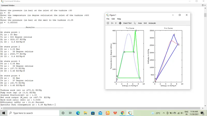
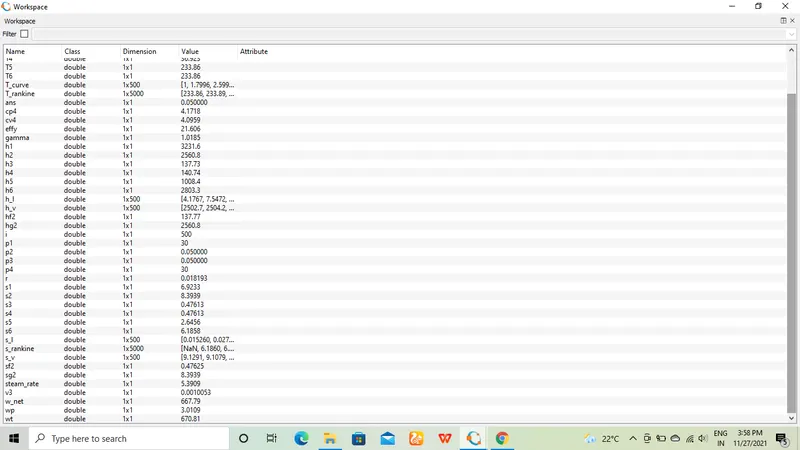
Workspace values.
Plots obtained.
2.Errors face while programming.
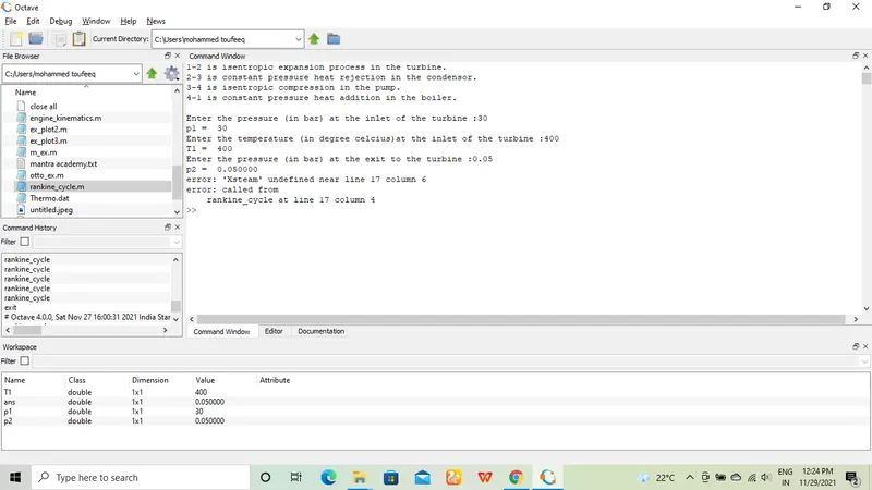
1.The following error appeared: "error: 'Xsteam' undefined near line 17 column 6
error: called from
rankine_cycle at line 17 column 4"
3.Screenshot below shows the error thrown in the command window.
4.Steps taken to rectify the errors.
The above mentioned error appeared becoz i mistakenly typed "Xsteam" instead of "XSteam" i.e letter s had to be in capital which was rectified later and the program ran successfully.
References: 1.https://skill-lync.com/student-projects/Rankine-cycle-Simulator-92065