Week 4.1 - Genetic Algorithm
The Genetic Algorithm is one of the 4 important classifications of the Evolutionary Algorithm, which are,
1. Genetic Algorithm(GA),
2. Differential Evolution (DE),
3. Evolution Strategies (ESs) and,
4. Estimation of Distribution Algorithms (EDAs).
Of which the GA is the only type that offers the best-optimized value that fits the solution results. Thus making a study on Genetic Algorithm is immensely important.
UNDERSTANDING THE GENETIC ALGORITHM:
WHAT IS GA?
A genetic algorithm is a method of solving and optimizing the results that mimic the biological evolution process which is imparted for searching and optimizing the desired functional values. The main concept behind it can be well explained with the Evolution process that has taken place and which is yet to occur, by the usage of chromosomes as the population and the characteristics of the population being controlled by the Genes for each of the Chromosomes.
EVOLUTION PROCESS:
First of all, we, in general, form a function that must have the desired number of genes that we wanted to be as unknowns. Let us take for example,
 , wherein a,b,c, and d are the genes.
The process takes place as in the flow chart given below.
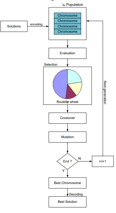
Biological Evolution is a 5 step process that involves the following,
- Initialization: In here the population (or) the no. of chromosomes are assumed, and hence giving random values for the genes which need not satisfy the desired function mentioned above.
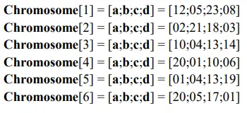
- Evaluation: In here we create the objective function values for each chromosome.
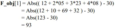 , where the objective function values of the other 5 chromosomes are similarly evaluated.
- Selection: In here the objective is to,
1. Select the fittest chromosome to make it available for the next upcoming generations.
2. Here, we formulate the Fitness value of each chromosome, with the help of which we calculate the Probability value for each chromosome, which predicts the chromosome with the highest probability that could make up to the next generation.
3. Then in order to form a Roulette wheel to make out random predictions of chromosomes we first formulate the cumulative probability values and then make the Roulette wheel which is shown below.
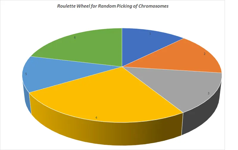
4. Then Random numbers are picked by spinning the Roulette wheel as 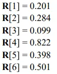 .
.
5. Then in comparison to the values we assign the newly formed chromosomes as,
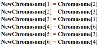
(Here the main takeaway is that the Chromosome 3 belongs to the 4th part of the pie-chart and hence is repeated twice, therefore, the higher the area, the higher is the probability for getting selected)
6. Thus the new set of chromosomes are formed on the above basis.
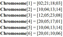
- Cross Over: Here we primarily fix the cross over rate value and then with the help of the Roulette wheel, we will again make random value generation and equate them to the newly formed chromosomes and find the ones that have the value lower than cross over rate and are made to cross over with themselves.
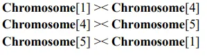
Thus leading to a new set of chromosomes which are given below.
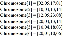
- Mutation: In a very similar way to that of the Cross Over, we do a step called the mutation, after which the objective function values for each of the chromosomes would have deceased values which means the convergence of the best genes for the next generation has been achieved for that particular iteration(single generation).
- Result: At last, after 50 similar iterations(50 generations), the optimized values of genes that best fits the function was found out to be,

The same is the way for optimizing any function with the help of a Genetic Algorithm and hence it always has its own unique importance in optimization.
(Reference:https://drive.google.com/file/d/1VZDVu0_PHIjHlz6CwSDcbznlC0C9DmFt/view?usp=sharing)
STALAGMITE FUNCTION AND ITS OPTIMIZATION:
A Stalagmite is a kind of rock formation from the floor of the caves that arises due to the accumulation of minerals during the dripping of water through the rock surfaces. Physically it has uneven peaks and troughs which can be made used to computationally represent the rises and falls for a given function(Eg. Food Supply over different regions, Climatic Conditions over different regions, Pressure variation, etc,.).
Let us see the step-wise coding for this challenge.
1. Creating 1,2-Dimensional x and y Arrays:
clear all
close all
clc

x=linspace(0,0.6,150);
y=linspace(0,0.6,150);
[xx,yy]=meshgrid(x,y); %Forming 2Dimensional array
Code Explanation:
- Here the CODE starts with the elementary codes clear all, close all, and clc followed by the creation of and y 1 Dimensional arrays and hence forming the 2 Dimensional arrays of x and y elements using the meshgrid command.
2. Creating the Function for Stalagmite creation:
The stalagmite model can be created with the help of the following equations, which are later imparted in MATLAB inside a function.
 ;
; 
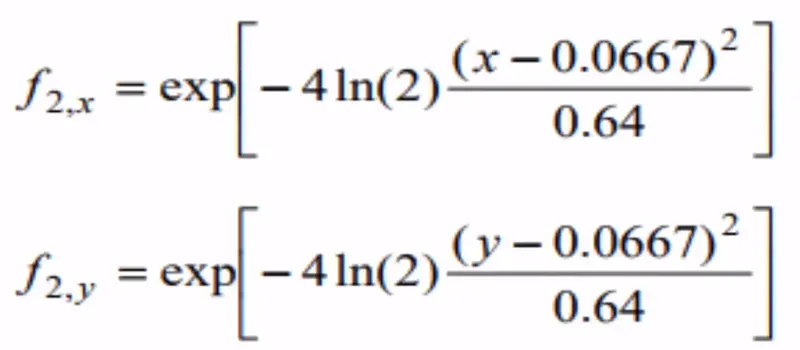
Here, the CODE for the Stalagmite creation is given below.
function [f]=stalagmite(inp)
    %Creation of Stalagmite Function:
    f1_x=(sin(5.1*pi*inp(1) + 0.5))^6;
    f1_y=(sin(5.1*pi*inp(2) + 0.5))^6;
    f21=(-4 * log(2) * (inp(1)-0.0667)^2)/0.64;
    f22=(-4 * log(2) * (inp(2)-0.0667)^2)/0.64;
    f2_x=exp(f21);
    f2_y=exp(f22);

    f=-(f1_x*f1_y*f2_x*f2_y);
end
Code Explanation:
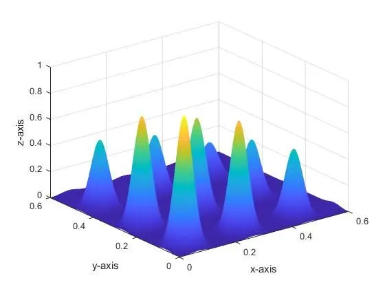
- Here the -ve sign is given for f in order to invert the stalagmite from upside down to top facing to represent the Maxima values since it is our objective to find the Global Maxima
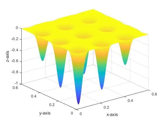 ==>
==>
- For which the input terms for the Stalagmite function are given from the main CODE as follows.
for i=1:length(xx)
    for j=1:length(yy)
        input_vector(1)=xx(i,j);
        input_vector(2)=yy(i,j);
        f(i,j)=stalagmite(input_vector);
    end
end
cases=170;
Code Explanation:
- The thing which we are doing here is first we are spreading out the sheet with x and y axes, with the inside plot values generated by the meshgrid command.
- Now using the for loop two times(x and y axes), we specify the value of each ordinate and abscissa in a 2-Dimensional form and impart those to the input_vector which is a single array consisting of 2 elements.
- Thus these x and y forms of input vectors are given as the input for the stalagmite function call.
- Here cases represent the number of iterations that we require for the Genetic algorithm to run.
From here, we will jump onto explore the three different study cases of the Genetic Algorithm's Optimization techniques.
#Study_Case_1:
%%

%Study 1:
%========
tic
for j=1:cases
    [opts1,fval1(j)]=ga(@stalagmite,2);
    xopt1(j)=opts1(1);
    yopt1(j)=opts1(2);
end

mean1=-(mean(fval1));

figure(1)
subplot(2,1,1)
hold on
surf(x,y,-f)
shading interp
plot3(xopt1,yopt1,-fval1,'marker','o','MarkerSize',5,'MarkerFaceColor','r')
xlabel('x-axis')
ylabel('y-axis')
title('Study Case 1')
subtitle('Stalagmite Model with Optimized points')
subplot(2,1,2)
plot(fval1)
subtitle('Functional Value through GA optimization Vs Iterations')
xlabel('Iterations')
ylabel('Function Value')

toc;
toc1=toc;
study_time1=toc1;
Code Explanation:
- The Genetic Algorithm method is deployed over the previously created Stalagmite function using the function handle command along with the number of variables given as input parameters as 2(x,y) for 170 iterations.
- In general, the Genetic Algorithm reduces the functional value over which it is employed and always finds the minimum value of the function.
- Thus we use an inverted stalagmite for the GA to calculate the minimum value at its upside-down facing bottom-most peak and then with the help of the -ve sign we just topple it to get it as a Global maxima value.
- Here, when we use the ga command it gives back the values of variables(x,y) and the functional value which are eventually stored in opts1(a 2 element single array) consisting of the x and y values and fval that consist of the functional value.
- Now the optimized functional value for their respective x and y points are thus created by the GA.
- In order to check for the correct optimization of the Functional values through GA, we check the mean of the functional values obtained.
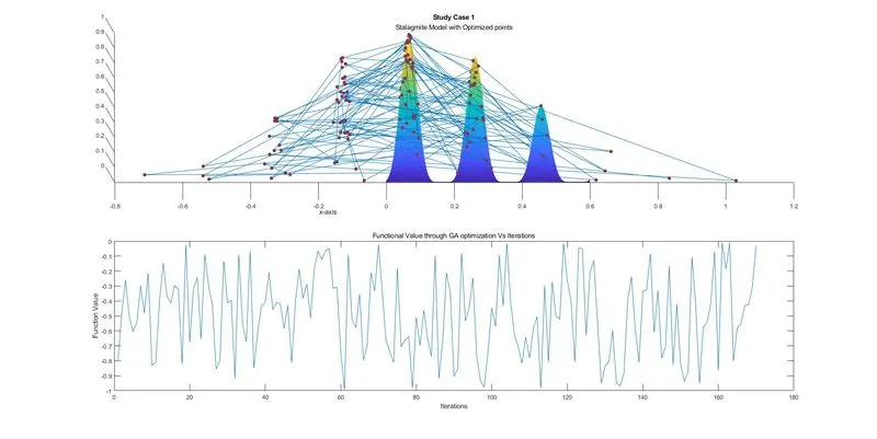
- Then we create 2 subplots, of which in the first one, we create a stalagmite model using the surf command, and using the plot3 command, we try to mark the GA optimized functional value after 170 iterations. And in the second plot, we determine the functional values optimized through the GA at each iteration by plotting a graph between them.
- The command shading interp is used to have a smooth contour on the surface of the stalagmite.
Result:
Inference:
- It can be seen that the GA performs its Optimization function out of the domain(x=0,y=0 to x=0.6,y=0.6) also, and has no fixed but various optimized function values for every iteration across and beyond the domain, which is not a good means of Optimization.
- The total run time taken for the GA to optimize the values for 170 iterations is 10 seconds.
- The mean value of the function must be 1 but in this case study, we are having the value of mean=0.4699
- Thus we now go for the next case study that involves the Boundedness condition.
#Study_Case_2:
%%
%Study 2:
%========
tic

for j=1:cases
    [opts2,fval2(j)]=ga(@stalagmite,2,[],[],[],[],[0,0],[0.6,0.6]);
    xopt2(j)=opts2(1);
    yopt2(j)=opts2(2);
end

mean2=-(mean(fval2));

figure(2)
subplot(2,1,1)
hold on
surf(x,y,-f)
shading interp
plot3(xopt2,yopt2,-fval2,'marker','o','MarkerSize',5,'MarkerFaceColor','r')
xlabel('x-axis')
ylabel('y-axis')
title('Study Case 2')
subtitle('Stalagmite Model with Optimized points')
subplot(2,1,2)
plot(fval2)
subtitle('Functional Value through GA optimization Vs Iterations')
xlabel('Iterations')
ylabel('Function Value')

toc;
toc2=toc;
study_time2=toc2;
Code Explanation:
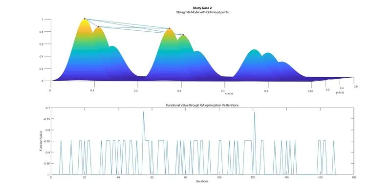
- This study is very similar to that of the first case but here we additionally involve the Boundedness condition for the GA to search for the minimum function value within the prescribed domain.
- Thus we use the x and y limits inside the ga command which is represented as,
x= ga(fun,nvars,A,b,Aeq,beq,lb,ub)x, so that a solution is found in the rangelb≤x≤ub. where A, B, Aeq, beq are the inequalities and equalities constraints that can b incorporated in the function if required. - But in here we neglect those constraints and concentrate only on the Boundedness condition lb and ub which are given the values of (lb(x=0,y=0) to ub(x=0.6,y=0.6)).
Result:
Inference:
- Here the GA almost optimizes the correct minimum values(here inverted into Global Maxima) when it is given with the Boundedness condition.
- But still, for the whole 170 iterations, it oscillates between 4 different minimum points which can be rectified by the usage of optimoptions condition which would be discussed in case 3.
- The total run time taken for the GA to optimize the values for 170 iterations is almost equal to 12 seconds.
- The mean value of the function must be 1 but in this case study, we are having the value of mean=0.9583
#Study_Case_3:
%%
%Study 3:
%========
tic

opt=optimoptions('ga');
opt=optimoptions(opt,'PopulationSize',700);
for j=1:cases
    [opts3,fval3(j)]=ga(@stalagmite,2,[],[],[],[],[0,0],[0.6,0.6],[],[],opt);
    xopt3(j)=opts3(1);
    yopt3(j)=opts3(2);
end

mean3=-(mean(fval3));

figure(3)
subplot(2,1,1)
hold on
surf(x,y,-f)
shading interp
plot3(xopt3,yopt3,-fval3,'marker','o','MarkerSize',5,'MarkerFaceColor','r')
xlabel('x-axis')
ylabel('y-axis')
title('Study Case 3')
subtitle('Stalagmite Model with Optimized points')
subplot(2,1,2)
plot(fval3)
subtitle('Functional Value through GA optimization Vs Iterations')
xlabel('Iterations')
ylabel('Function Value')

toc;
toc3=toc;
study_time3=toc3;
Code Explanation:
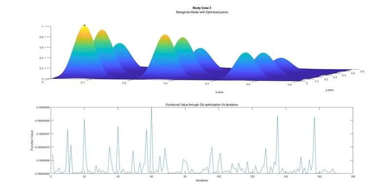
- This study is very similar to case study 2, but what we mainly include here is increasing the population size so that the optimization becomes more accurate at the end of each iteration(Because as the population increases there will also be better chances for an increase in the count of fittest chromosomes(in terms of Biological Evolution)).
- Thus we use the optimoptions command to optimize the through the GA for increased population size and include it in the GA function as, [opts3,fval3(j)]=ga(@stalagmite,2,[],[],[],[],[0,0],[0.6,0.6],[],[],opt).
Result:
Inference:
- Hence the accurate result through the GA-based optimization has been obtained pointing towards the minimum most point(here inverted into Global Maxima) for each and every iteration.
- The mean value of the function must be 1 but in this case study, we are having the value of mean=1.
- The total run time taken for the GA to optimize the values for 170 iterations is almost equal to 109.82 seconds which is a bit higher due to the increase in population size.
The full MATLAB CODE is pasted below.
FULL PROGRAM:
clear all
close all
clc

x=linspace(0,0.6,150);
y=linspace(0,0.6,150);
[xx,yy]=meshgrid(x,y); %Forming 2Dimensional array

for i=1:length(xx)
    for j=1:length(yy)
        input_vector(1)=xx(i,j);
        input_vector(2)=yy(i,j);
        f(i,j)=stalagmite(input_vector);
    end
end
cases=170;
%%

%Study 1:
%========
tic
for j=1:cases
    [opts1,fval1(j)]=ga(@stalagmite,2);
    xopt1(j)=opts1(1);
    yopt1(j)=opts1(2);
end

mean1=-(mean(fval1));

figure(1)
subplot(2,1,1)
hold on
surf(x,y,-f)
shading interp
plot3(xopt1,yopt1,-fval1,'marker','o','MarkerSize',5,'MarkerFaceColor','r')
xlabel('x-axis')
ylabel('y-axis')
title('Study Case 1')
subtitle('Stalagmite Model with Optimized points')
subplot(2,1,2)
plot(fval1)
subtitle('Functional Value through GA optimization Vs Iterations')
xlabel('Iterations')
ylabel('Function Value')

toc;
toc1=toc;
study_time1=toc1;

%%
%Study 2:
%========
tic

for j=1:cases
    [opts2,fval2(j)]=ga(@stalagmite,2,[],[],[],[],[0,0],[0.6,0.6]);
    xopt2(j)=opts2(1);
    yopt2(j)=opts2(2);
end

mean2=-(mean(fval2));

figure(2)
subplot(2,1,1)
hold on
surf(x,y,-f)
shading interp
plot3(xopt2,yopt2,-fval2,'marker','o','MarkerSize',5,'MarkerFaceColor','r')
xlabel('x-axis')
ylabel('y-axis')
title('Study Case 2')
subtitle('Stalagmite Model with Optimized points')
subplot(2,1,2)
plot(fval2)
subtitle('Functional Value through GA optimization Vs Iterations')
xlabel('Iterations')
ylabel('Function Value')

toc;
toc2=toc;
study_time2=toc2;

%%
%Study 3:
%========
tic

opt=optimoptions('ga');
opt=optimoptions(opt,'PopulationSize',700);
for j=1:cases
    [opts3,fval3(j)]=ga(@stalagmite,2,[],[],[],[],[0,0],[0.6,0.6],[],[],opt);
    xopt3(j)=opts3(1);
    yopt3(j)=opts3(2);
end

mean3=-(mean(fval3));

figure(3)
subplot(2,1,1)
hold on
surf(x,y,-f)
shading interp
plot3(xopt3,yopt3,-fval3,'marker','o','MarkerSize',5,'MarkerFaceColor','r')
xlabel('x-axis')
ylabel('y-axis')
title('Study Case 3')
subtitle('Stalagmite Model with Optimized points')
subplot(2,1,2)
plot(fval3)
subtitle('Functional Value through GA optimization Vs Iterations')
xlabel('Iterations')
ylabel('Function Value')

toc;
toc3=toc;
study_time3=toc3;
FUNCTION:
function [f]=stalagmite(inp)
    %Creation of Stalagmite Function:
    f1_x=(sin(5.1*pi*inp(1) + 0.5))^6;
    f1_y=(sin(5.1*pi*inp(2) + 0.5))^6;
    f21=(-4 * log(2) * (inp(1)-0.0667)^2)/0.64;
    f22=(-4 * log(2) * (inp(2)-0.0667)^2)/0.64;
    f2_x=exp(f21);
    f2_y=exp(f22);

    f=-(f1_x*f1_y*f2_x*f2_y);
end
FINAL RESULTS:
CONCLUSION:
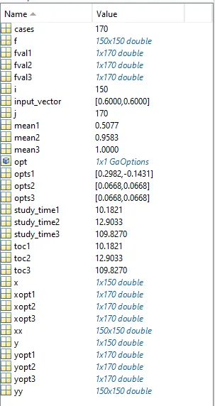
The #Study_Case_3 gave the best results in terms of optimization through the Genetic Algorithm by solving within the designated boundaries and also optimizing the function by increasing the population size and thus having the mean of the functional value almost equal to 1 but only with the additional drawback of time expenditure compared to the next best yielding case 2.