Challenge

Genetic Algorithm

HHansel Kirk Kullu9 Nov 2021

AIM: To write a program in MATLAB, to optimize the stalagmite function and find the global maxima of the function.

OBJECTIVE:

Explain the concept as well as the syntax of genetic algorithm.

THEORY:

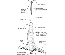
A stalagmite is an upward-growing mound of mineral deposits that have precipitated from water dripping onto the ocean floor of a cave. Most stalagmites have rounded or flattened tips.

A Genetic Algorithm (GA) is a method for solving both constrained and unconstrained optimization problems based on a natural selection process that mimics biological evolution. The algorithm repeatedly modifies a population of individual solutions. At each step, the genetic algorithm randomly selects individuals from the current population and uses them as parents to produce the children for the next generation. Over successive generations, the population "evolves" toward an optimal solution.

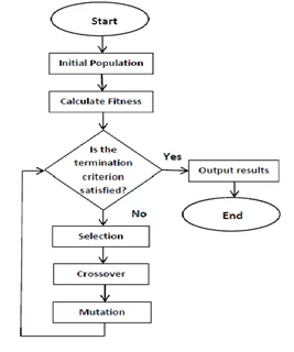
Basic Terminologies:

Population: This is a subset of all the probable solutions that can solve the given problem.

Chromosomes: A chromosome is one of the solutions in the population.

Gene: This is an element in a chromosome.

Allele: This is the value given to a gene in a specific chromosome.

Fitness function: This is a function that uses a specific input to produce an improved output. The solution is used as the input while the output is in the form of solution suitability.

Genetic operators: In genetic algorithms, the best individuals mate to reproduce an offspring that is better than the parents. Genetic operators are used for changing the genetic composition of this next generation.

Syntax:

x = ga(fitnessfcn,nvars)

Finds a local unconstrained minimum, x, to the objective function, fitnessfcn. nvars is the dimension (number of design variables) of fitnessfcn.

x = ga(fitnessfcn,nvars,A,b)

Finds a local minimum x to fitnessfcn, subject to the linear inequalities A*x ≤ b. ga evaluates the matrix product A*x as if x is transposed (A*x').

x = ga(fitnessfcn,nvars,A,b,Aeq,beq)

Finds a local minimum x to fitnessfcn, subject to the linear equalities Aeq*x = beq as well as A*x ≤ b. (Set A=[] and b=[] if no linear inequalities exist.) ga evaluates the matrix product Aeq*x as if x is transposed (Aeq*x').

x = ga(fitnessfcn,nvars,A,b,Aeq,beq,LB,UB)

Defines a set of lower and upper bounds on the design variables, x, so that a solution is found in the range LB ≤ x ≤ UB. (Set Aeq=[] and beq=[] if no linear equalities exist.)

x = ga(fitnessfcn,nvars,A,b,Aeq,beq,LB,UB,nonlcon)

Subjects the minimization to the constraints defined in nonlcon. The function nonlcon accepts x and returns vectors Cand Ceq, representing the nonlinear inequalities and equalities respectively. ga minimizes the fitnessfcn such that C(x) ≤ 0 and Ceq(x) = 0. (Set LB=[] and UB=[] if no bounds exist.)

x = ga(fitnessfcn,nvars,A,b,Aeq,beq,LB,UB,nonlcon,options)

Minimizes with the default optimization parameters replaced by values in the structure options, which can be created using the gaoptimset function. (Set nonlcon=[] if no nonlinear constraints exist.)

x = ga(fitnessfcn,nvars,A,b,[],[],LB,UB,nonlcon,IntCon)

Requires that the variables listed in IntCon take integer values.

x = ga(fitnessfcn,nvars,A,b,[],[],LB,UB,nonlcon,IntCon,options)

Minimizes with integer constraints and with the default optimization parameters replaced by values in theoptions structure.

x = ga(problem)

Finds the minimum for problem, where problem is a structure.

[x,fval] = ga(fitnessfcn,nvars,...)

Returns fval, the value of the fitness function at x.

[x,fval,exitflag] = ga(fitnessfcn,nvars,...)

Returns exitflag, an integer identifying the reason the algorithm terminated.

[x,fval,exitflag,output] = ga(fitnessfcn,nvars,...)

Returns output, a structure that contains output from each generation and other information about the performance of the algorithm.

[x,fval,exitflag,output,population] = ga(fitnessfcn,nvars,...)

Returns the matrix, population, whose rows are the final population.

[x,fval,exitflag,output,population,scores] = ga(fitnessfcn,nvars,...)

Returns scores the scores of the final population.

EQUATION:

`f=f_1.f_2.f_3.f_4`

Where,

`f_1=(sin⁡(5.1πx+0.5))^6`

`f_2=(sin⁡(5.1πy+0.5))^6`

`f_3=exp[-4ln⁡(2)(x-0.0667)^2/0.64]`

`f_4=exp[-4ln⁡(2)(y-0.0667)^2/0.64]`

PROGRAM:

Function:

function [f]=stalagmite(input_vector)

 

x=input_vector(1);

y=input_vector(2);

f1=(sin(5.1*pi*x+0.5))^6;

f2=(sin(5.1*pi*y+0.5))^6;

f3=exp(-4*log(2)*(x-0.0667)^2/0.64);

f4=exp(-4*log(2)*(y-0.0667)^2/0.64);

 

f=-(f1*f2*f3*f4);

 

end

Explanation:

We first define the function stalagmite using the formula mentioned above.

Program:

clear all

close all

clc

 

x=linspace(0,0.4,150);

y=linspace(0,0.4,150);

num_cases=50;

 

 

%Creating a 2D mesh

[xx yy]=meshgrid(x,y);

 

%Evaluating the stalagmite function

for i=1:length(xx)

    for j=1:length(yy)

        input_vector(1)=xx(i,j);

        input_vector(2)=yy(i,j);

        f(i,j)=stalagmite(input_vector);

    end

end

 

%% Study-1

tic

 

%Study1-Statistical behavior

for i=1:num_cases

    [inputs1,fopt1(i)]=ga(@stalagmite,2);

    xopt1(i)=inputs1(1);

    yopt1(i)=inputs1(2);

end

 

study1_time=toc

 

%plot-1

figure(1)

subplot(2,1,1)

hold on

surfc(x,y,f)

shading interp

plot3(xopt1,yopt1,fopt1,'marker','o','markersize',5,'markerfacecolor','g')

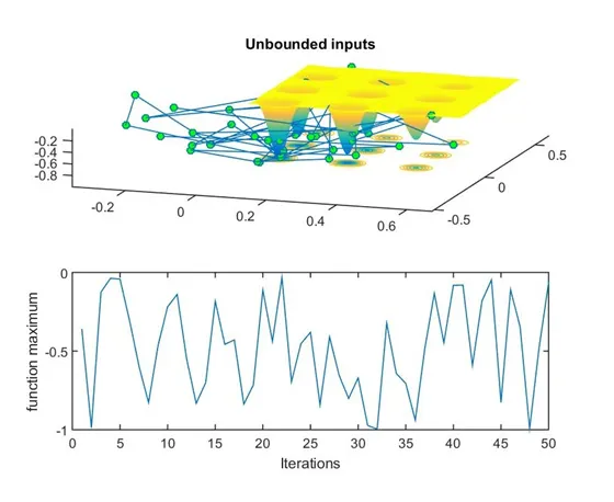
title('Unbounded inputs – Case 1')

subplot(2,1,2)

plot(fopt1)

xlabel('Iterations')

ylabel('function maximum')

 

%% Study-2

tic

 

%Study2-Statistical behavior-with upper and lower bounds

for i=1:num_cases

    [inputs2,fopt2(i)]=ga(@stalagmite,2,[],[],[],[],[0;0],[0.4;0.4]);

    xopt2(i)=inputs2(1);

    yopt2(i)=inputs2(2);

end

 

study2_time=toc

 

%plot-2

figure(2)

subplot(2,1,1)

hold on

surfc(x,y,f)

shading interp

plot3(xopt2,yopt2,fopt2,'marker','o','markersize',5,'markerfacecolor','r')

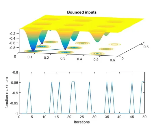
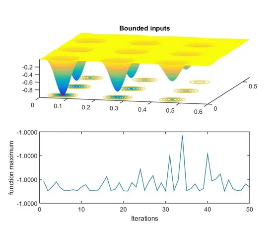
title('Bounded inputs')

subplot(2,1,2)

plot(fopt2)

xlabel('Iterations')

ylabel('function maximum')

 

%% Study-3

 

%increasing ga iteration

options=optimoptions('ga');

options=optimoptions(options,'populationsize',170);

tic

 

%Study3-Statistical behavior-with upper and lower bounds + options

for i=1:num_cases

    [inputs3,fopt3(i)]=ga(@stalagmite,2,[],[],[],[],[0;0],[0.4;0.4],[],[],options);

    xopt3(i)=inputs3(1);

    yopt3(i)=inputs3(2);

end

 

study3_time=toc

 

%plot-3

figure(3)

subplot(2,1,1)

hold on

surfc(x,y,f)

shading interp

plot3(xopt3,yopt3,fopt3,'marker','o','markersize',5,'markerfacecolor','r')

title('Bounded inputs')

subplot(2,1,2)

plot(fopt3)

xlabel('Iterations')

ylabel('function maximum')

Explanation:

We first begin with clear all, close all, clc to get rid of any previous data.
150 values from 0 to 0.4 are stored in x and y. The total number of cases is defined to be 50.
Then a 2D grid is created from the values stored in x and y using meshgrid
The stalagmite function is evaluated by running two for loops and using the generated values to be used as input for the stalagmite function.
For the first study of statistical behavior we initiate the timer using tic and toc command to calculate the time taken for the study. For loop is used to iterate the total number of cases thus calculating and storing the values in the variables. The results are then plotted.
For the second study, upper and lower bounds are introduced and the method of calculating the results are similar to the first study. Then the results are plotted.
For the third study, the population size is increased to 170 and calculated to plot the results.