Week 4.1 - Genetic Algorithm

A genetic algorithm is a metaheuristic inspiried by the process of natural selection that belongs to the larger class of evolutinory algorithms. Genetic algorithm are commonly used to generate high quality solution solution to optimization and search problems by reling on biologically inspired operators such as mitation, crossover and selection.

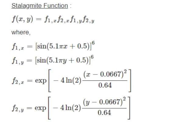
these function are use for plotting a fittest graph in main function.

function [f] = stalagmite_fun(input_vector)

f1x = (sin((5.1*pi).*input_vector(1)+0.5)).^6;
f1y = (sin((5.1*pi).*input_vector(2)+0.5)).^6;

f2x=exp((((input_vector(1)-0.0667).^2)/0.64).*(-4*log(2)));
f2y=exp((((input_vector(2)-0.0667).^2)/0.64).*(-4*log(2)));
f1=f1x*f1y**f2x*f2y;
f=-f1;
end

while using the function at the end we used -ve sign so that by using the plot we can find the maxima of the given function by ga.

*Main Coding

firstly making a one diamensional array of x and y

creating a two diamentional array of these two vector with the help of 'meshgrid' command.and define the number of iterations so we get best result.

now we calculate the fittest value of the function at each point of meshgrid format.

now creating the surface by using the 'surf'comand it also provide the contour on the generated surface.

while using the surf appling '-'sign function will generate the graph upside down which will a quite good to analyze the maxima.

clear all
close all
clc
% Definite our search space
x = linspace(0,0.6,150);
y = linspace(0,0.6,150);

% Creating a 2 Diamensional mesh
[xx yy] = meshgrid(x,y);

% Evaluating a stalagmite function
for i = 1:length(xx)

for j = 1:length(yy)
input_vector(1)=xx(i,j)
input_vector(2)=yy(i,j);
f(i,j)=stalagmite(input_vector);

end

end

surf(xx,yy,-f) % generating the surfacexlabel('x axis')
ylabel('y axis')
zlabel('z axis')
shading interp % to removing the lines on the graph
[x,f]= ga(@stalagmite,2)

% the plot generated show down below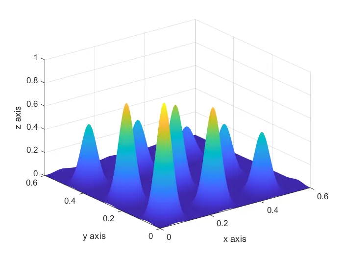

% STATISTICAL BEHAVIOUR (UNBOUNDED).

clear all
close all
clc
% Definite our search space
x = linspace(0,0.6,150);
y = linspace(0,0.6,150);
iterations = 50;
% Creating a 2 Diamensional mesh
[xx yy] = meshgrid(x,y);

% Evaluating a stalagmite function
for i = 1:length(xx)

for j = 1:length(yy)
input_vector(1)=xx(i,j);
input_vector(2)=yy(i,j);
f(i,j)=stalagmite(input_vector);

end

%% STATISTICAL BEHAVIOUR UNBOUNDED

end

% % studing the statiscial behaviour of GA
tic
for i=1:iterations
[input , fopt(i)] = ga(@stalagmite,2);
xopt(i) = input(1);
yopt(i) = input(2);
end

iteration_1_time = toc

%plotting
figure (1)
subplot(2,1,1)
hold on
surfc(xx,yy,f);
shading interp
plot3(xopt,yopt,fopt,'marker','o','markersize',5,'markerfacecolor','r')
subplot(2,1,2)
plot(fopt)
xlabel('iterations')
ylabel('function minimum')

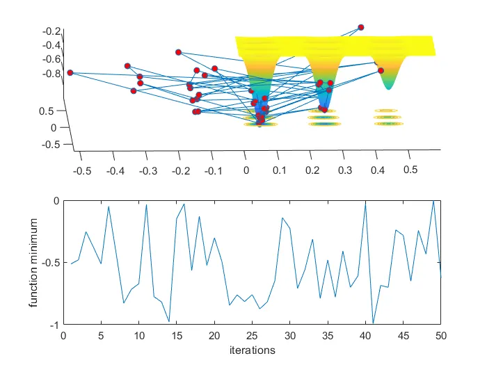
* Above figure shows that result are not much accurate and giving a lot of variation in optimizing the function.

*STATISTIC STUDY WITH BOUNDATION

• Here we provide a upper and lower limit so that search space is reduced with the upper and lower boundry.

and plotting the same code.

tic
% stastical behaviour with upper and lower bounds

for i=1:iterations
[input2 , fopt2(i)] = ga(@stalagmite,2,[],[],[],[],[0;0],[1;1]); % calculating the optimized value at each itteration of bound
xopt2(i) = input2(1);
yopt2(i) = input2(2);
end
toc
iteration_2_time = toc

%plotting
figure (2)
subplot(2,1,1)
hold on
surfc(xx,yy,f);
shading interp
plot3(xopt2,yopt2,fopt2,'marker','o','markersize',5,'markerfacecolor','r')
subplot(2,1,2)
plot(fopt2)
xlabel('iterations')
ylabel('function minimum')

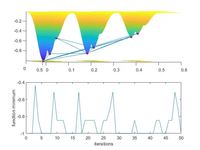
*It is clearly seen that in above figure by putting the upper limit the variation are reduced.

%STATISTICAL STUDY WITH INCREASING IN POPULATION

• In this study using 'optimoption' command to increse the size of population.
• the benifit of that it will working a large number of set and it will be lead to find the fittest function value. but it will take more time compare to both of above. % study 3
  % increasing GA population
  tic

options = optimoptions ('ga');
options = optimoptions(options,'populationsize',500);

for i=1:iterations
[input2 , fopt3(i)] = ga(@stalagmite,2,[],[],[],[],[0;0],[1;1],[],[],options); % increasing the size of function

by using 'optimoption' function

xopt3(i) = input2(1);
yopt3(i) = input2(2);
end
toc
iteration_3_time = toc

%plotting
figure (3)
subplot(2,1,1)
hold on
surfc(xx,yy,f);
shading interp
plot3(xopt3,yopt3,fopt3,'marker','o','markersize',5,'markerfacecolor','r')
xlabel('x');
ylabel('y')
subplot(2,1,2)
plot(fopt3)
xlabel('iterations')
ylabel('function minimum')

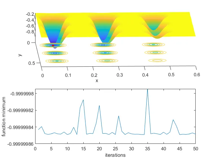
% RESULT

Here we get a accurate value by reducing the error.