Week 4.1 - Genetic Algorithm

Genetic Algorithm (stalagmite):

Aim:

1. To show how the global maxima obtains in stalagmite function using 'Genentic Algorithm'.
2. Plotting graphs to show how the function maximum changes with multiple iterations.

Theory:

In genetic algorithm, generally the term 'Algorithm' refers,

Algorithm:

An algorithm is a step procedure to solve logical and mathematical problems. A recipe is a good example of an algorithm because it says what must be done, step by step. It takes inputs (ingredients) and produces an output (the complete dish).

Genetic Algorithm:

It is a machine learning algorithm used to find optimized (suitable) results for complex problems.

- introduced by charles darwin in 1975.

- provides efficient, effective techniques for optimization and machine learning applications.

- reflects the process of natural selection where the fittest individuals (variables) are selected for reproduction in order to produce offspring of the next generation.

- widely used today in business, scientific & engineering circles.

Flowchart of 'GA':

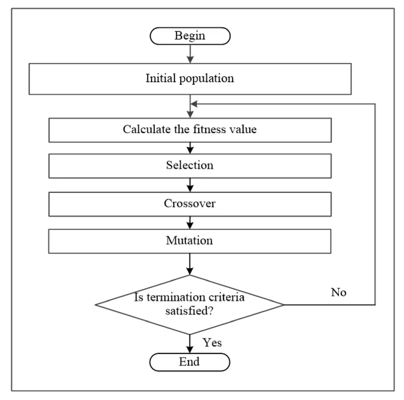
5 stages of Genetic Algorithm are:

1. Initial population: Every individual who are involved in the process are called population. Defining every individual as variables.
2. Calculate fitness: Calculates the fitness value for the given population (variables). It determines how fit the individual is.
3. Selection: It is a process of selecting where the individual with highest fitness value.
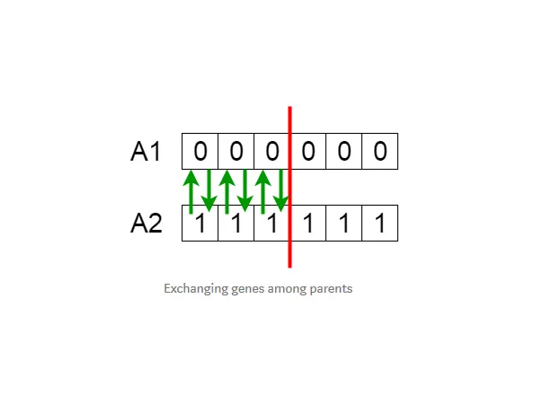
4. Cross over: Selected pair of strings is cut at some random positions & these segments are swapped to form new pair of strings.

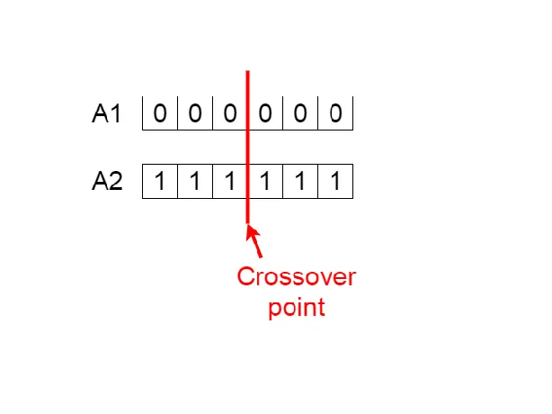
offspring are generated by exchanging genes among parents.

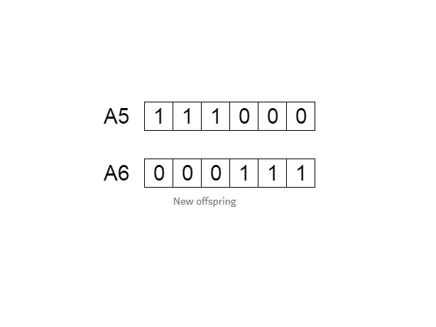
The new off springs are produced

v. Mutation: Mutation is done to maintain diversity with the population and to prevent the occurance of a convergence prematurely.

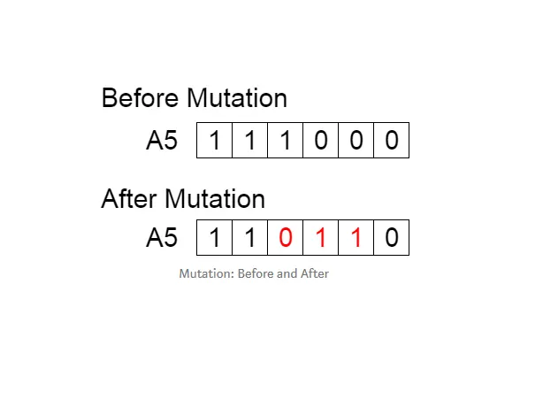
The alogrithm terminates once the convergence is obtained.

*In this project we're going to discuss about stalagmite using 'Genetic Algorithm'.

Stalagmite:

A stalagmite is a type of rock formation that rises from the floor of a cave due to the accumulation of material deposited on the floor from ceiling drippings.

- typically composed of calcium carbonate, but may consist of lava, mud, peat, sand, sinter and amberat.

The following is the given stalagmite function for which we need to find the global maxima.

Function of stalagmite:

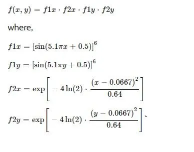
Code of the function in MATLAB:

% Creating a stalagmite function for genetic algorithm

function [f] = stalagmite(input_vector)

x = input_vector(1);
y = input_vector(2);
f1_x = (sin(5.1*pi*x + 0.5))^6;
f1_y = (sin(5.1*pi*y + 0.5))^6;

f2_x = exp(-4*log(2)*(x-0.0667)^2/0.64);
f2_y = exp(-4*log(2)*(y-0.0667)^2/0.64);

f = -(f1_x*f1_y*f2_x*f2_y);

end

Procedure:

1. Initially stalagmite is defined in function and later it is called into the main program.
2. A negative sign is used in the code for 'z value' to obtain maxima of the function rather than minima.
3. A nested for loop is utilized to iterate each of the elements.
4. By using 'tic' & 'toc' commands, the times of each cases in the program are measured.
5. 'GA' is used to determine the optimal of the function.
6. Plot is generated for different cases.

The three cases considered are:

i. Unbounded inputs.

ii. Bounded inputs - restricted with upper and lower bounds (so the search space is minimized).

iii. Bounded inputs - increasing no. of iterations by giving population size.

Explaination of syntax for GA:

x = ga(fun,nvars)

x = ga(fun,nvars,A,B)

x = ga(fun,nvars,A,B,Aeq,Beq)

x = ga(fun,nvars,A,b,Aeq,Beq,lb,ub)

x = ga(fun,nvars,A,b,Aeq,Beq,lb,ub,nonlcon)

x = ga(fun,nvars,A,b,Aeq,Beq,lb,ub,nonlcon,options)

x = ga(fun,nvars,A,b,[],[],lb,ub,nonlcon,IntCon)

x = ga(fun,nvars,A,b,[],[],lb,ub,nonlcon,IntCon,options)

x = ga(problem)

[ x, fval ] = ga(______)

Here Input Arguments are:

fun - objective function

nvars - no. of variables

A - linear inequality constraints

B - linear inequality constraints

Aeq - linear equality constraints

Beq - linear equality constraints

lb - lower bound

ub - upper bound

nonlcon - nonlinear constraints

IntCon - integer variables

options - optimization options

problem - problem descriptions

Output Arguments:

x - Solution.

fval - Objective function value at the solution.

CODE FOR STALAGMITE USING 'GA':

clear all
close all 
clc

% Creating stalagmite using MATLAB


% Creating a 1D array for x & y values
x = linspace(0,0.6,150);
y = linspace(0,0.6,150);

% Creating a 2D array using meshgrid for 'stalagmite'
[xx,yy] = meshgrid(x,y);

% Using 'forloop' to get different outputs of Z
for i = 1:length(xx)
    for j = 1:length(yy)
    input_vector(1) = xx(i,j);
    input_vector(2) = yy(i,j);
    f(i,j) = stalagmite(input_vector);
    
    end
end
    
% Plotting the    
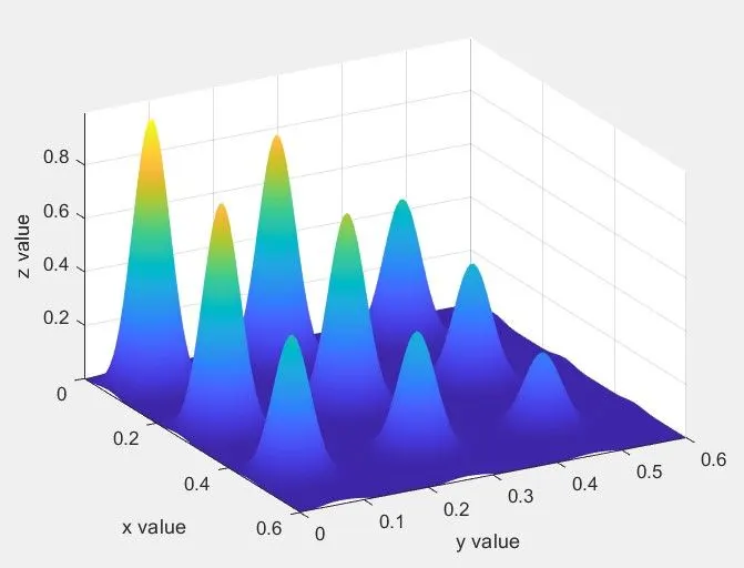
surfc(xx,yy,-f)
xlabel('x value')
ylabel('y value')
zlabel('z value')
shading interp

% Using 'Genetic Algorithm' for optimised results
[results, fval] = ga(@stalagmite, 2)

Output:

Resluts in command window:

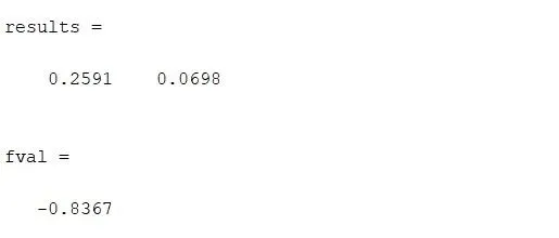
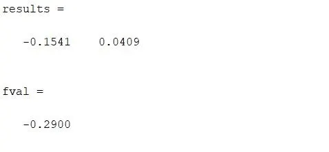
*when you run the GA code for a single time, the optimum value (result) for the function obtains.

*These optimum results changes whenever you run the code, So its better to take multiple iterations to show the most optimum result in the function. As the GA command used does not identify iteration, it must do in a search space, a variable called as 'iterations' is defined and the value is set as '50'.

*So, for a better understanding we're going to define multiple iterations to run the code. The results are plotted in a graph inorder to show where the optimum value of the function lies.

The three cases considered are:

i. Unbounded inputs.

ii. Bounded inputs - restricted with upper and lower bounds (so the search space is minimized).

iii. Bounded inputs - increasing no. of iterations by giving population size.

MAIN PROGRAM:

clear all
close all 
clc

% Creating stalagmite using MATLAB


% Creating a 1D array for x & y values
x = linspace(0,0.6,150);
y = linspace(0,0.6,150);

% Creating a 2D array using meshgrid for 'stalagmite'
[xx,yy] = meshgrid(x,y);

% Using 'forloop' to get different outputs of Z
for i = 1:length(xx)
    for j = 1:length(yy)
    input_vector(1) = xx(i,j);
    input_vector(2) = yy(i,j);
    f(i,j) = stalagmite_function(input_vector);
    
    end
end

% Three diff cases are plotted below:

iterations = 50;

%--------------------------------------------------------------------------------
% Case 1


% Case1: searching for optimum results without search space (unbounded inputs)

tic

for i = 1:iterations
    [inputs,f_optimum(i)] = ga(@stalagmite_function,2);
    x_optimum(i) = inputs(1);
    y_optimum(i) = inputs(2);
end

toc
case1_time = toc

figure(1)
subplot(2,1,1)
surfc(xx,yy,-f)
xlabel('x value')
ylabel('y value')
zlabel('z value')
title('Case1: Unbounded inputs')
shading interp
hold on
plot3(x_optimum,y_optimum,-f_optimum,'marker','o','markersize',5,'markerfacecolor','r')
subplot(2,1,2)
plot(-f_optimum)
xlabel('Iterations')
ylabel('F maximum')


%-----------------------------------------------------------------------------------
% Case 2


% Case2: searching within a search space (bounded inputs)
 
tic

for i = 1:iterations
    [inputs,f_optimum(i)] = ga(@stalagmite_function,2,[],[],[],[],[0;0],[0.6;0.6]);
    x_optimum(i) = inputs(1);
    y_optimum(i) = inputs(2);
end

toc
case2_time = toc

figure(2)
subplot(2,1,1)
surfc(xx,yy,-f)
xlabel('x value')
ylabel('y value')
zlabel('z value')
title('Case2: Bounded inputs')
shading interp
hold on
plot3(x_optimum,y_optimum,-f_optimum,'marker','o','markersize',5,'markerfacecolor','r')
subplot(2,1,2)
plot(-f_optimum)
xlabel('Iterations')
ylabel('F maximum')


%------------------------------------------------------------------------------------
% Case 3


% Case3: Increasing the population size & optimizing the results

% 'options' is used for optimizing the results with increasing population
options = optimoptions('ga');
options = optimoptions(options,'PopulationSize',350);

tic

for i = 1:iterations
    [inputs,f_optimum(i)] = ga(@stalagmite_function,2,[],[],[],[],[0,0],[0.6,0.6],[],[],options);
    x_optimum(i) = inputs(1);
    y_optimum(i) = inputs(2);
end

toc
case3_time = toc

figure(3)
subplot(2,1,1)
surfc(xx,yy,-f)
xlabel('x value')
ylabel('y value')
zlabel('z value')
title('Case3: Bounded inputs with population')
shading interp
hold on
plot3(x_optimum,y_optimum,-f_optimum,'marker','o','markersize',5,'markerfacecolor','r')
subplot(2,1,2)
plot(-f_optimum)
xlabel('Iterations')
ylabel('F maximum')

OUTPUT:

Case 1 & Case 2:

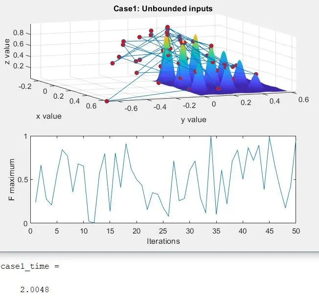
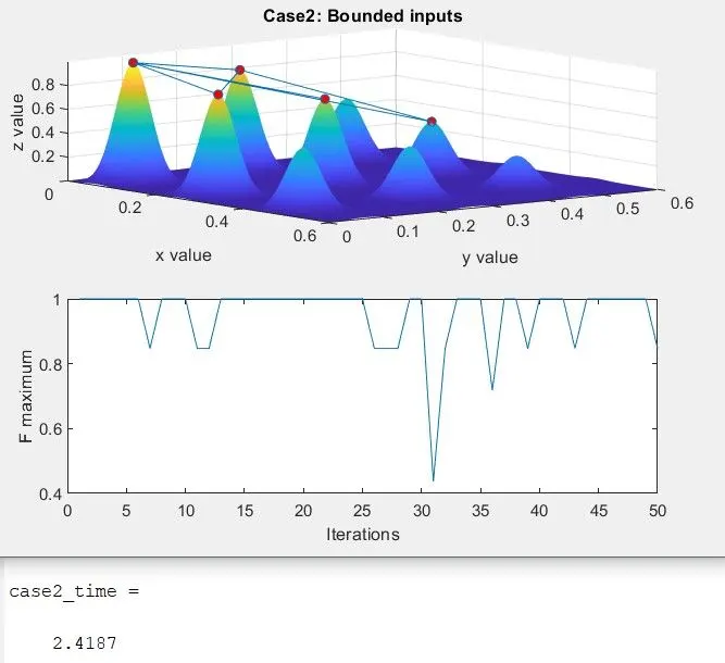
Case 3:

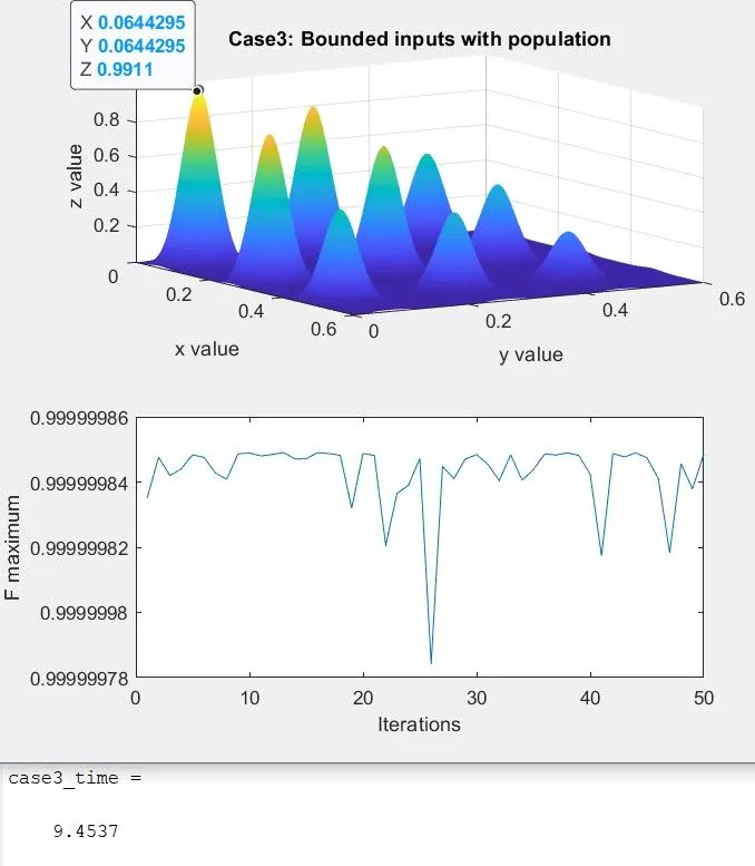
CONCLUSION:

1. The process of obtaining global maxima has been done.
2. 'GA' uses the technique of optimization that finding the best solution from the different no. of solutions.
3. It's better to assign search space that GA does not consider any particular search space to obtain optimum results.