Week 4.1 - Genetic Algorithm

AIM:

1. To write a code in MATLAB to optimise the stalagmite function and find the global maxima of the function.
2. To expalin the concept of genetic algorithm in your own words and also explain the syntax for ga in MATLAB in your report.
3. The code scripted should gives the same output, though it is made to run several times.
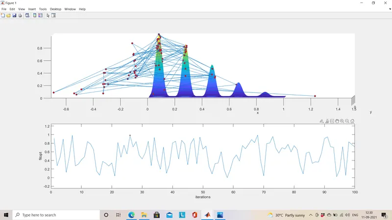
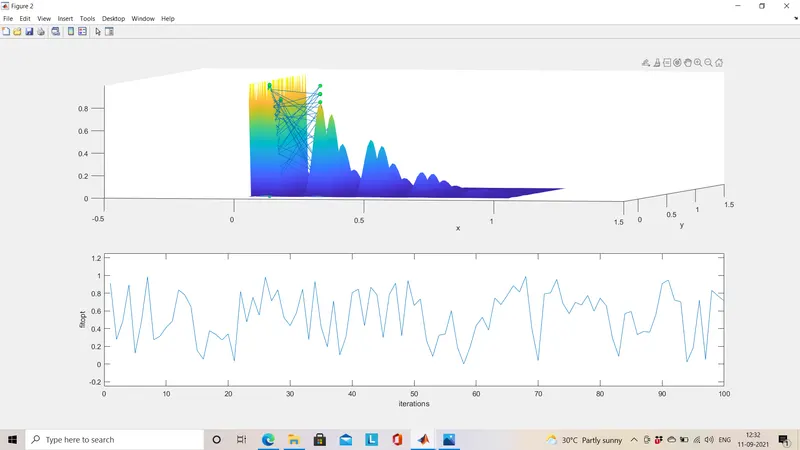
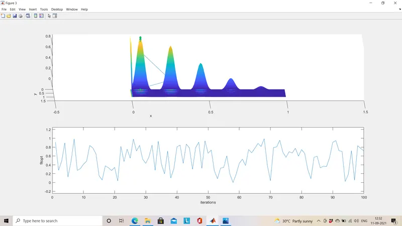
4. To Plot the graphs for all three studies and for F maximum vs no. of iterations

GENETIC ALGORITHM:

Genetic algorithms are a biomimic type of optimization algorithm, meaning they are used to find the maximum or minimum of a function.This concept is proposed by charles darwin in19th century.Genetic algorithms represent one branch of the field of study called evolutionary computation, in that they imitate the biological processes of reproduction and natural selection to solve for the ‘fittest’ solutions . Like in evolution, many of a genetic algorithm’s processes are random, however this optimization technique allows one to
set the level of randomization and the level of control . These algorithms are far more powerful and efficient than random search and exhaustive search algorithms , yet require no extra information about the given problem. This feature allows them to find solutions to problems that other optimization methods cannot handle due to a lack of continuity, derivatives, linearity, or other features.

i)Components, Structure, & Terminology
Since genetic algorithms are designed to simulate a biological process, much of the relevant terminology is borrowed from biology. However, the entities that this terminology refers to in genetic algorithms are much simpler than their biological counterparts . The basic components common to almost all genetic algorithms are:

• a fitness function for optimization

• a population of chromosomes

• selection of which chromosomes will reproduce

• crossover to produce next generation of chromosomes

• random mutation of chromosomes in new generation

uses:

In the present day, genetic algorithms are used by large companies to optimize schedules and design products that range from large aircraft to tiny computer chips to medicines.

The Los Alamos National Laboratory has used them to analyze the data from satellites .They were used to create realistic special effects for films like Troy and The Lord of the Rings

There are also many applications for genetic algorithms in the financial sector, such as identifying fraud and predicting market fluctuations. They are even being used in the development new forms of art and music

Parallel computing has made genetic algorithms even more appealing because it can alleviate their main drawback: the lack of speed.

syntax of ga:

x = ga(fun,nvars)

Finds a local unconstrained minimum, x, to the objective function, fun. nvars is the dimension (number of design variables) of fun.

x = ga(fun,nvars,A,b)

x = ga(fun,nvars,A,b) finds a local minimum x to fun, subject to the linear inequalities A*x ≤ b. ga evaluates the matrix product A*x as if x is transposed (A*x').

x = ga(fun,nvars,A,b,Aeq,beq)

x = ga(fun,nvars,A,b,Aeq,beq) finds a local minimum x to fun, subject to the linear equalities Aeq*x = beq and A*x ≤ b. (Set A=[] and b=[] if no linear inequalities exist.)
ga evaluates the matrix product Aeq*x as if x is transposed (Aeq*x').

x = ga(fun,nvars,A,b,Aeq,beq,lb,ub)

x = ga(fun,nvars,A,b,Aeq,beq,lb,ub) defines a set of lower and upper bounds on the design variables, x, so that a solution is found in the range lb ≤ x ≤ ub.
(Set Aeq=[] and beq=[] if no linear equalities exist.)

x = ga(fun,nvars,A,b,Aeq,beq,lb,ub,nonlcon)

x = ga(fun,nvars,A,b,Aeq,beq,lb,ub,nonlcon) subjects the minimization to the constraints defined in nonlcon. The function nonlcon accepts x and returns vectors C and Ceq, representing the nonlinear inequalities and equalities respectively.
ga minimizes the fun such that C(x) ≤ 0 and Ceq(x) = 0. (Set lb=[] and ub=[] if no bounds exist.)

x = ga(fun,nvars,A,b,Aeq,beq,lb,ub,nonlcon,options)

x = ga(fun,nvars,A,b,Aeq,beq,lb,ub,nonlcon,options) minimizes with the default optimization parameters replaced by values in options. (Set nonlcon=[] if no nonlinear constraints exist.) Create options using optimoptions.

x = ga(fun,nvars,A,b,[],[],lb,ub,nonlcon,IntCon)

x = ga(fun,nvars,A,b,[],[],lb,ub,nonlcon,IntCon) or x = ga(fun,nvars,A,b,[],[],lb,ub,nonlcon,IntCon,options) requires that the variables listed in IntCon take integer values.

x = ga(fun,nvars,A,b,[],[],lb,ub,nonlcon,IntCon,options)

x = ga(problem)

x = ga(problem) finds the minimum for problem, a structure described in problem.

[x,fval] = ga(___)

[x,fval] = ga(___), for any previous input arguments, also returns fval, the value of the fitness function at x.

[x,fval,exitflag,output] = ga(___)

[x,fval,exitflag,output] = ga(___) also returns exitflag, an integer identifying the reason the algorithm terminated, and output, a structure that contains output from each generation and other information about the performance of the algorithm.

[x,fval,exitflag,output,population,scores] = ga(___)

[x,fval,exitflag,output,population,scores] = ga(___) also returns a matrix population, whose rows are the final population, and a vector scores, the scores of the final population.

here we use command 4 and 5 to get bounded inputs and increased population size

syntax for 'option' command used for increasing the population size

options = optimoptions(@ga)

The option can be used to change the default value to desired value.

This returns options with the default values for its fields. ga uses these default values if you do not pass in options as an input argument.

The value of each option is stored in a field of options, such as options.PopulationSize.
You can display any of these values by entering options followed by a period and the name of the field.
For example, to display the size of the population for the genetic algorithm.

CODE SCRIPTED IN MATLAB:

#main program to find global maxima:

clear all
close all
clc

%creating array of numbers using linspace command 

x= linspace(0,1,100);

y = linspace(0,1,100);

[xx yy] = meshgrid(x,y); %meshgrid used to create two-D array

for i = 1:100
    for j = 1:100
        ip(1) = xx(i,j);
        ip(2) = yy(i,j);
        fit(i,j) = stalagmite(ip);
    end
end
       
num = 100;
%%case - 1 with unbounded inputs:
tic  %command used to measure the processing time
for i = 1:num
    [i_p,fitopt(i)] = ga(@stalagmite,2); %this ga identifies minimum value for the function without any boundary limits
    
    %optimum value of x & y
    xopt(i) = i_p(1);
    
    yopt(i) = i_p(2);
end

toc

figure(1)

subplot(2,1,1)
hold on
 %To find global maxima we use negative value
surfc(xx,yy,-fit) 
shading interp     %this command is used to remove the grid lines in the surfc diagram

plot3(xopt,yopt,-fitopt,'marker','o','markersize',5,'markerfacecolor','r')
xlabel('x')
ylabel('y')
axis([-0.5 1.5 -0.25 1.5 0 0.8])
subplot(2,1,2)

plot(-fitopt) 
xlabel('iterations')
ylabel('fitopt')
axis([0 100 -0.25 1.25])

%%case-2 with bounded inputs:

tic
for i =  1:num
    [i_p,fit(i)] = ga(@stalagmite,2,[],[],[],[],[0;0],[0.5;0.5]); % the ga command here used to find the minimum value for the function 
    xopt(i) = i_p(1);
    yopt(i) = i_p(2);
end
toc

figure(2)

subplot(2,1,1)
hold on
%To find global maxima we use negative value
surfc(x,y,-fit)
shading interp     %this command is used to remove the grid lines in the surfc diagram

plot3(xopt,yopt,-fitopt,'marker','o','markersize',5,'markerfacecolor','g')
xlabel('x')
ylabel('y')
axis([-0.5 1.5 -0.25 1.5 0 0.8])
subplot(2,1,2)

plot(-fitopt) %
xlabel('iterations')
ylabel('fitopt')
axis([0 100 -0.25 1.25])

%%case-3 with increased population size:

options = optimoptions('ga','populationsize',300); %option command here used to change the population size from default value

tic
for i = 1:num
    [i_p,fit(i)] = ga(@stalagmite,2,[],[],[],[],[0;0],[1;1],[],options);
    xopt(i) = i_p(1);
    yopt(i) = i_p(2);
end
    toc
    
figure(3)

subplot(2,1,1)
hold on
surfc(x,y,-fit) %To find global maxima we use negative value
shading interp

plot3(xopt,yopt,-fitopt,'marker','o','markersize',5,'markerfacecolor','g')
xlabel('x')
ylabel('y')
axis([-0.5 1.5 -0.25 1.5 0 0.8])
subplot(2,1,2)

plot(-fitopt) %
xlabel('iterations')
ylabel('fitopt')
axis([0 100 -0.25 1.25])

%%saving the plot automatically

saveas(figure(1),'plot with unbounded inputs.jpg')
saveas(figure(2),'plot with bounded inputs.jpg')
saveas(figure(3),'plot with increased pop size.jpg')

#function code for stalagmite:

function [fit] = stalagmite(ip)
x =ip(1);
y= ip(2);
%%function we are going to find global maxima

f1x = (sin((5.1*pi*x)+0.5))^6;
f2x = exp(-4*log(2)*((x-0.0667)^2)/0.64);
f1y = (sin((5.1*pi*y)+0.5))^6;
f2y =  exp(-4*log(2)*((y-0.0667)^2)/0.64);
fit = -(f1x*f2x*f1y*f2y);

end

Code explainaton:

COMMANDS USED(NEW):

meshgrid - The command is used to create two dimensional array from the 1D array,syntax:[xx yy] = meshgrid(x,y) where x and y is one dimensional array.

ga - This is the command for genetic algorithm which is the in built-in function whose types of syntax is defined above.

tic-toc - It is the command used to calculate the processing time of a operation,the operation where we need the processing time should be written/scripted within the tic and toc.

surfc - The surfc command is used to create three dimensional surface plot with colors peak region is depicted in different color having syntax : surfc(x,y,z)

shading interp - The shading interp command is used to remove the grid lines in the surface plot and make them neat ,this command is written after the surface plot.

plot3 - plot3(x,y,z) plots coordinates in 3-D space.It plot multiple sets of coordinates on the same set of axes, specify at least one of X, Y, or Z as a matrix and the others as vectors.

subplot - subplot(m,n,p) divides the current figure into an m-by-n grid and creates axes in the position specified by p. The first subplot is the first column of the first row, the second subplot is the second column of the first row, and so on. If axes exist in the specified position, then this command makes the axes the current axes.

saveas - The saveas command is used to save the plot,surfaceplot automatically while the code is running in the folder where the program is stored we can change the folder by using mkdir,cd.

options - This option is used to differ from default value which is in the old position to be replaced with the new value.

$$ Function code:

1. We start the program using defining function where it has two inputs x and y
2. The function has four unknown f1x,f2x,f1y,f2y they are defined with the given formula.
3. Then defining function by multiplying the unknowns and multiply them with negative value since the given funciton gives minimum value.make sure you end the function.

$$ Main code:

• We initiate the main code with clearing and closing previous commands.
• Then we create two different one dimensional array, after that two dimensional array is created using meshgrid command.
• For loop is created with the population size as its limit and calling the funtion to run.
• Then three cases are coded to get the maximum value of the function.First case is done with unbounded inputs.
• Second case is done with bounded inputs so that the function get the maximum limit within that range.We set a limit for lower bound and upper bound for x and y.
• Third case is done with increased population size.we write the function with negative value so that it can get global maxima since 'ga' command get only the minimum value.
• plot3 command is used to plot three values which are optimised value derived from the function .
• In the third case we use a command 'option' which is used to change the default value with the new value using optimoption tool.
• After finding the function value we plot the graph for maximum function value and the number of iterations for the three studies or cases.
• Each case or study is plotted in different figure ,each figure has two plots one is surface plot another is maximum value plot to get that we use subplot.
• Then we use save as command is used to save the plot while the code is executing.

PLOT IMAGES:

This below image depicts the plot for the unbounded inputs condition where we have a clumpsy graph.

This below image depicts the plot for the bounded inputs condition where the maximum function value range is reduced compared to previous one.

This below image depicts the plot for the increased population size condition where the maximum function value range is much reduced.By increasing the iteration or population size we can get the best fit value so far.The processing time will also increase.

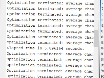
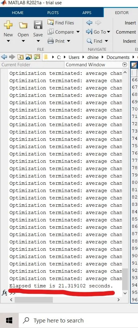
PROCESSING TIME IMAGES:

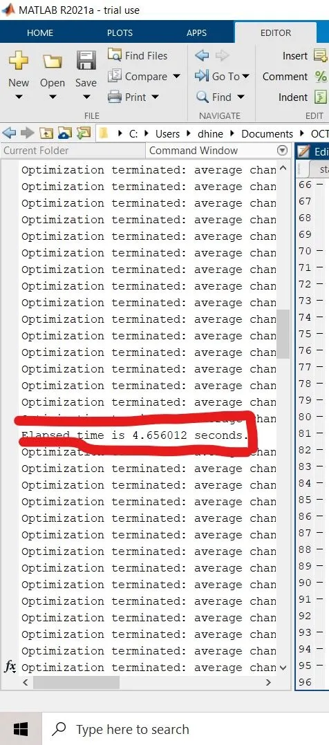
The processing time increases from one case to other case1<case2<case3.

CONCLUSION:

1. The code to find the global maxima of the given function is written and executed successfully.
2. Genetic algorithm definition,uses and its syntax is explained.
3. plotting of maximum function value verse iteration is done.

REFERENCE:

GA Selection operators (iitg.ac.in)

http://www.flll.jku.at/div/teaching/Ga/GA-Notes.pdf

Find minimum of function using genetic algorithm - MATLAB ga - MathWorks India