Week 4.1 - Genetic Algorithm
"Week 4.1 - Genetic Algorithm"
Aim:
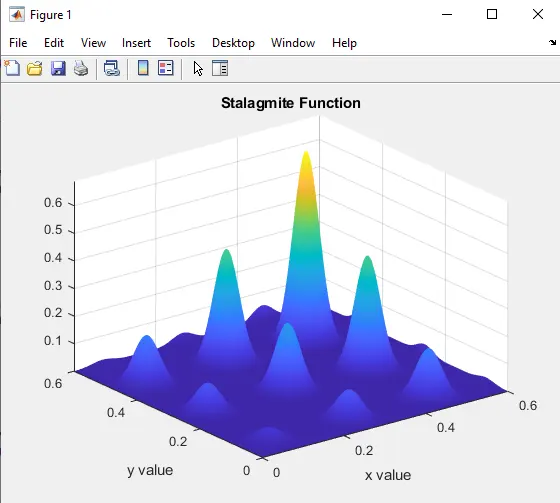
To write a code in Matlab to optimize the stalagmite function and find the global maxima of the function.
Objective:
- To write a code in MATLAB to optimize the stalagmite function and to find the global maxima of the function.
- To explain the concept of genetic algorithm in my own words and also to explain the syntax for ga in MATLAB.
- To plot graphs for all 3 studies and for F maximum vs no. of iterations.
Optimization:
Optimization is an act or methodology of making something as fully perfect, functional, or effective as possible. The purpose of optimization is to achieve the best design relative to set prioritized criteria or constraints. These include maximizing factors such as productivity, strength, reliability, longevity, efficiency, and utilization.
Mathematical Optimization:
Mathematical optimization (alternatively spelled optimization) or mathematical programming is the selection of the best element, with regard to some criterion, from some set of available alternatives. Optimization problems of sorts arise in all quantitative disciplines from computer science and engineering to operations research and economics, and the development of solution methods has been of interest in mathematics for centuries.
In the simplest case, an optimization problem consists of maximizing or minimizing a real function by systematically choosing input values from within an allowed set and computing the value of the function. The generalization of optimization theory and techniques to other formulations constitutes a large area of applied mathematics. More generally, optimization includes finding "best available" values of some objective function given a defined domain (or input), including a variety of different types of objective functions and different types of domains.
Stalagmite function:
It is a function that contains the input parameters that are to be given plot like stalagmite structure. Calling the function stalagmite that contains the code for evaluates the value of the function using the array input. For the study of the statistical behavior of the Genetic Algorithm, primarily a stopwatch is started.
It contains the following formulas to generate the data that cause to be plot,
`F = (F1x*F1y*F2x*F2y)`
`F1y = (sin(5.1*pi*y1 + 0.05))^6`
`F2x = exp(-4*log(2)*((x1- 0.0667)^2/0.64))`
`F2y = exp(-4*log(2)*((y1- 0.0667)^2/0.64))`
Genetic Algorithm:
The genetic algorithm is a method for solving both constrained and unconstrained optimization problems that is based on natural selection, the process that drives biological evolution. The genetic algorithm repeatedly modifies a population of individual solutions. At each step, the genetic algorithm selects individuals at random from the current population to be parents and uses them to produce the children for the next generation. Over successive generations, the population "evolves" toward an optimal solution. You can apply the genetic algorithm to solve a variety of optimization problems that are not well suited for standard optimization algorithms, including problems in which the objective function is discontinuous, nondifferentiable, stochastic, or highly nonlinear. The genetic algorithm can address problems of mixed integer programming, where some components are restricted to be integer-valued.
The genetic algorithm uses three main types of rules at each step to create the next generation from the current population:
-
Selection rules select the individuals, called parents, that contribute to the population at the next generation.
-
Crossover rules combine two parents to form children for the next generation.
-
Mutation rules apply random changes to individual parents to form children.
A genetic algorithm is a search heuristic that is inspired by Charles Darwin’s theory of natural evolution. This algorithm reflects the process of natural selection where the fittest individuals are selected for reproduction in order to produce offspring of the next generation.
Notion of Natural Selection
The process of natural selection starts with the selection of fittest individuals from a population. They produce offspring which inherit the characteristics of the parents and will be added to the next generation. If parents have better fitness, their offspring will be better than parents and have a better chance at surviving. This process keeps on iterating and at the end, a generation with the fittest individuals will be found.
This notion can be applied for a search problem. We consider a set of solutions for a problem and select the set of best ones out of them.
Five phases are considered in a genetic algorithm.
- Initial population
- Fitness function
- Selection
- Crossover
- Mutation
Initial Population
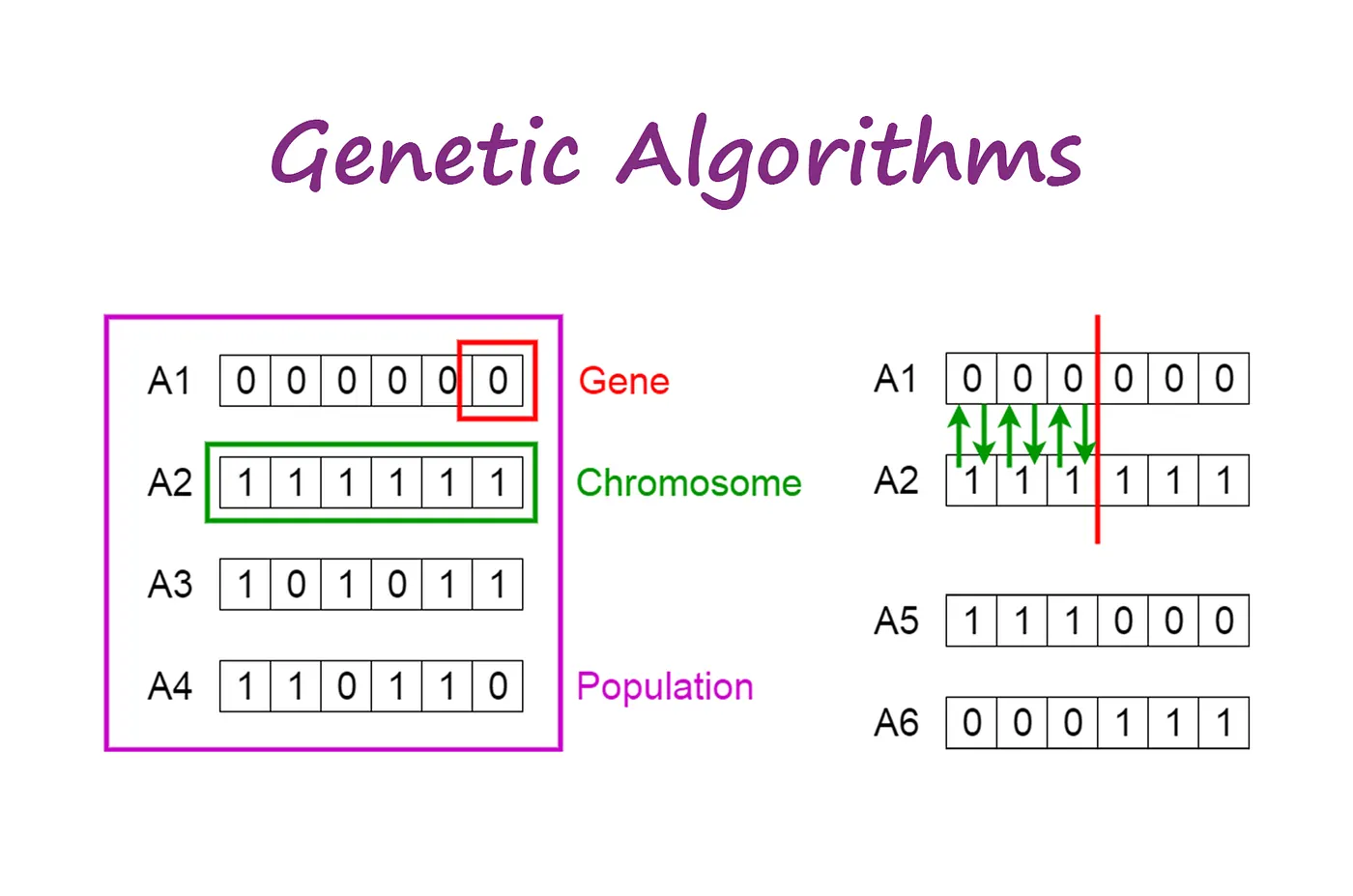
The process begins with a set of individuals which is called a Population. Each individual is a solution to the problem you want to solve.
An individual is characterized by a set of parameters (variables) known as Genes. Genes are joined into a string to form a Chromosome (solution).
In a genetic algorithm, the set of genes of an individual is represented using a string, in terms of an alphabet. Usually, binary values are used (string of 1s and 0s). We say that we encode the genes in a chromosome.
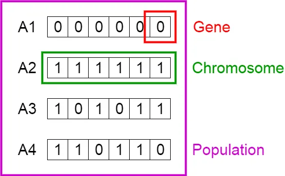
Population, Chromosomes and Genes
Fitness Function
The fitness function determines how fit an individual is (the ability of an individual to compete with other individuals). It gives a fitness score to each individual. The probability that an individual will be selected for reproduction is based on its fitness score.
Selection
The idea of selection phase is to select the fittest individuals and let them pass their genes to the next generation.
Two pairs of individuals (parents) are selected based on their fitness scores. Individuals with high fitness have more chances to be selected for reproduction.
Crossover
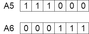
Crossover is the most significant phase in a genetic algorithm. For each pair of parents to be mated, a crossover point is chosen at random from within the genes.
For example, consider the crossover point to be 3 as shown below.
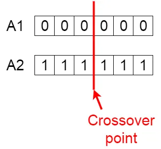
Crossover point
Offspring are created by exchanging the genes of parents among themselves until the crossover point is reached.
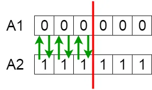
Exchanging genes among parents
The new offspring are added to the population.
New offspring
Mutation
In certain new offspring formed, some of their genes can be subjected to a mutation with a low random probability. This implies that some of the bits in the bit string can be flipped.
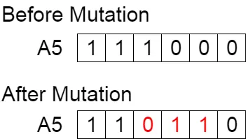
Mutation: Before and After
Mutation occurs to maintain diversity within the population and prevent premature convergence.
Termination
The algorithm terminates if the population has converged (does not produce offspring which are significantly different from the previous generation). Then it is said that the genetic algorithm has provided a set of solutions to our problem.
GA is a function of Matlab
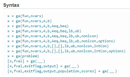
Descriptions:
x = ga(fun,nvars) finds a local unconstrained minimum, x, to the objective function, fun. nvars is the dimension (number of design variables) of fun.
Note:-
Passing Extra Parameters explains how to pass extra parameters to the objective function and nonlinear constraint functions, if necessary.
x = ga(fun,nvars,A,b) finds a local minimum x to fun, subject to the linear inequalities A*x ≤ b. ga evaluates the matrix product A*x as if x is transposed (A*x').
x = ga(fun,nvars,A,b,Aeq,beq) finds a local minimum x to fun, subject to the linear equalities Aeq*x = beq and A*x ≤ b. (Set A=[] and b=[] if no linear inequalities exist.) ga evaluates the matrix product Aeq*x as if x is transposed (Aeq*x').
x = ga(fun,nvars,A,b,Aeq,beq,1b,ub) defines a set of lower and upper bounds on the design variables, x, so that a solution is found in the range lb ≤ x ≤ ub. (Set Aeq=[] and beq=[] if no linear equalities exist.)
x = ga(fun,nvars,A,b,Aeq,beq,1b,ub,nonlcon) subjects the minimization to the constraints defined in nonlcon. The function nonlcon accepts x and returns vectors C and Ceq, representing the nonlinear inequalities and equalities respectively. ga minimizes the fun such that C(x) ≤ 0 and Ceq(x) = 0. (Set lb=[] and ub=[] if no bounds exist.)
x = ga(fun,nvars,A,b,Aeq,beq,1b,ub,nonlcon,options)minimizes with the default optimization parameters replaced by values in options. (Set nonlcon=[] if no nonlinear constraints exist.) Create options using optimoptions.
x = ga(fun,nvars,A,b,[],[],1b,ub,nonlcon,IntCon,options) or x = ga(fun,nvars,A,b,[],[],lb,ub,nonlcon,IntCon,options)IntCon take integer values.
Note:-
When there are integer constraints, ga does not accept linear or nonlinear equality constraints, only inequality constraints.
x = ga(problem) finds the minimum for problem, a structure described in problem.
[x,fval] = ga(___), for any previous input arguments, also returns fval, the value of the fitness function at x.
[x,fval,exitflag,output] = ga(___) also returns exitflag, an integer identifying the reason the algorithm terminated, and output, a structure that contains output from each generation and other information about the performance of the algorithm.
[x,fval,exitflag,output,population,scores] = ga(___)also returns a matrix population, whose rows are the final population, and a vector scores, the scores of the final population.
Matlab Main Program:
close all
clear all
clc

% Defining our search space
x = linspace(0,0.6,150);
y = linspace(0,0.6,150);

% Creating a  2-D Mesh
[xx,yy] = meshgrid(x,y);

% Evaluating the stalagmite function
for i = 1:length(xx)
    for j = 1:length(yy)
        input_vector(1) = xx(i,j);
        input_vector(2) = yy(i,j);
        F(i,j) = stalagmite_function(input_vector);
    end
end
% Plotting The Graph
figure(1)

surfc(xx,yy,-F)
shading interp
xlabel('x value')
ylabel('y value')
title('Stalagmite_Function')

% Study 1
n_iteration = 50;
tic
for i = 1:n_iteration
    [inputs_a,Fopt_a(i)] = ga(@stalagmite_function,2);
    xopt1(i) = inputs_a(1);
    yopt1(i) = inputs_a(2);
    clc
end
study_time1 = toc
% Plotting the Graph
figure(2)
subplot(2,1,1)
hold on
surfc(x,y,F)
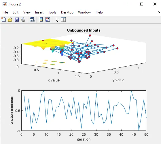
title('Unbounded Inputs')
xlabel('x value')
ylabel('y value')
shading interp
hold on
plot3(xopt1,yopt1,Fopt_a,'marker','o','markersize',5,'markerfacecolor','r')
subplot(2,1,2)
plot(Fopt_a)
xlabel('iteration')
ylabel('function minimum')
tic

% Study 2 - statistical behavior with upper and lower bounds
for i = 1:n_iteration
    [inputs_b,Fopt_b(i)] = ga(@stalagmite_function,2,[],[],[],[],[0;0],[0.6;0.6]);
    xopt(i) = inputs_b(1);
    yopt(i) = inputs_b(2);
    clc
end
study2_time = toc
% Plotting The Graph
figure(3)
subplot(2,1,1)
surfc(x,y,F)
shading interp
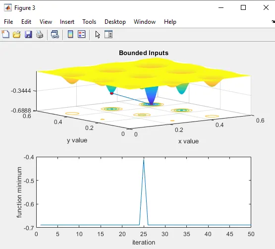
title('Bounded Inputs')
xlabel('x value')
ylabel('y value')
hold on
plot3(xopt1,yopt1,Fopt_b,'marker','o','markersize',5,'markerfacecolor','r')
subplot(2,1,2)
plot(Fopt_b)
xlabel('iteration')
ylabel('function minimum')

% Study 3 - Increasing the population size
options = optimoptions(@ga);
options = optimoptions(@ga,'populationsize',200);
tic
for i = 1:n_iteration
    [inputs_c,Fopt_c(i)] = ga(@stalagmite_function,2,[],[],[],[],[0;0],[0.6;0.6],[],[],options);
    xopt(i) = inputs_c(1);
    yopt(i) = inputs_c(2);
    clc
end
study3_time = toc
figure(4)
subplot(2,1,1)
surfc(x,y,F)
shading interp
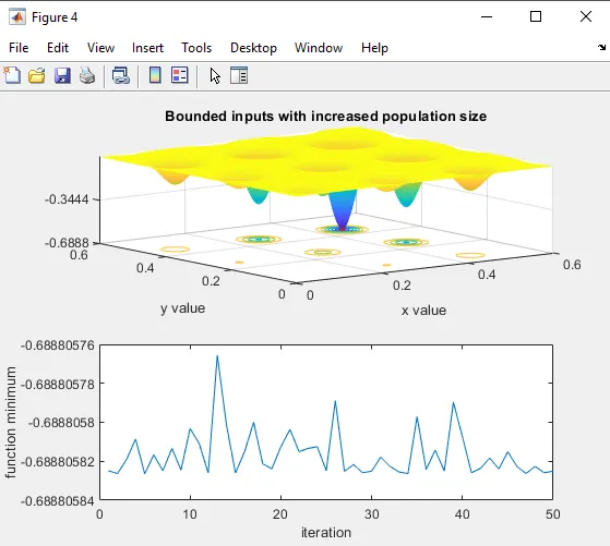
title('Bounded inputs with increased population size')
xlabel('x value')
ylabel('y value')
hold on
plot3(xopt1,yopt1,Fopt_c,'marker','o','markersize',5,'markerfacecolor','r')
subplot(2,1,2)
plot(Fopt_c)
xlabel('iteration')
ylabel('function minimum')
Program Explanation:
- At first two inputs are given namely x & y.
- Then by using the 'linspace' command we set the data between two numbers.
- Next, by using the 'meshgrid' command we created an array of m*n matrix.
- By using for loop operation
The input vector stored the value of matrix xx & yy and the output vector was stored in the 'F' matrix after evaluated of stalagmite function.
- Then we have used surf(x,y,z) command to create the 3-d surface plot with a contour plot underneath. Surface plot is a 3-d surface that has edge color & solid surface color.
- After that label command was used to label the axis of the graph.
- Next, we have used 'shading interp' to hide the grid and to get the graph smooth.
- ## Study - 1 in genetic algorithm of random sampling
In this case, we have taken the no. of iteration 50.
- Then ##Study - 2 statistical behavior with upper and lower bounds and ## Study - 3 Increasing the population size was calculated and also the no. of iteration was taken in Study - 2 and Study - 3 50.
- we have used 'tic toc' command in all the cases to calculate the time running.
Matlab Function Code:
function[F] = stalagmite_function(input_vector)

% Defining input conditions
x = input_vector(1);
y = input_vector(2);

% Solving the equations to obtain the values of the function
f1x = (sin((5.1*pi*x)+0.5))^6;
f1y = (sin((5.1*pi*y)+0.5))^6;
f2x = exp(-4*log(2)*(((x-0.667)^2)/0.64));
f2y = exp(-4*log(2)*(((y-0.667)^2)/0.64));
F = -(f1x*f1y*f2x*f2y);
end
Result:
1) Stalagamite Function:-
2) Unbounded Inputs:-
3) Bounded Inputs:-
4) Bounded inputs with increased population size:-
Errors Encountered:
1)
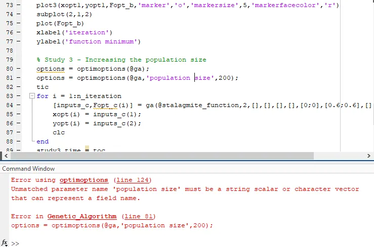
From the above picture, we can clearly see that we have given space between population and size. In Matlab, population size is one word. So, to execute the code we have removed the space between population and size and made it a one-word 'populationsize'.
2)
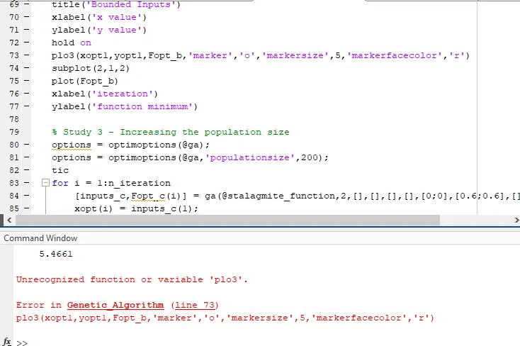
From the above picture, we can clearly see that there was some typos mistake in line no. 73. So, to execute the code we have corrected the 'plo3' to 'plot3'.
Conclusion:
We have studied the concept of Genetic Algorithm and optimized the Stalagmite Function in Matlab.
References:
2) https://in.mathworks.com/help/gads/what-is-the-genetic-algorithm.html