Genetic Algorithm
AIM: To write a code in MATLAB to optimize the stalagmite function and find the global maxima of the function.
THEORY: Genetic Algorithm
A genetic algorithm (GA) is a method for solving both constrained and unconstrained optimization problems based on a natural selection process that mimics biological evolution. It is a model or abstraction of biological evolution based on Charles Darwin's theory of natural selection. These genetic operators, the crossover and recombination, mutation, and selection in the study of adaptive and artificial systems form the essential part of the genetic algorithm as a problem-solving strategy.
There are many advantages of genetic algorithms over traditional optimization algorithms. The two most notable are: the ability to deal with complex problems and parallelism. Genetic algorithms can deal with various types of optimization, whether the objective (fitness) function is stationary or non-stationary (change with time), linear or nonlinear, continuous or discontinuous, or with random noise. Because multiple offsprings in a population act like independent agents, the population (or any subgroup) can explore the search space in many directions simultaneously. This feature makes it ideal to parallelize the algorithms for implementation. Different parameters and even different groups of encoded strings can be manipulated at the same time.
However, genetic algorithms also have some disadvantages. The formulation of the fitness function, the use of population size, the choice of the important parameters such as the rate of mutation and crossover, and the selection criteria of the new population should be carried out carefully. Any inappropriate choice will make it difficult for the algorithm to converge or it will simply produce meaningless results. Despite these drawbacks, genetic algorithms remain one of the most widely used optimization algorithms in modern nonlinear optimization.
Genetic algorithms have increasingly been applied in engineering in the past decade, due to it is considered as a tool for optimization in engineering design. This work introduces the use of genetic algorithms to solve complex optimization problems, manage the uncertainty in typical industrial scenarios. In this context, this work uses the GA as an optimization tool for decision making to determine the optimal production, inventory level, and distribution in the Supply Chain planning problem under uncertainty. A MILP stochastic approach has been solved using a generic genetic algorithm of Matlab obtaining improved solutions.
Since the solution obtained has a good performance in time/quality of the results for the proposed model. This work determines that new schemes of genetic algorithms are an opportunity for future extensions of its capability for more complex models as recursive stochastic approaches and nonlinear models.
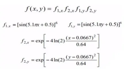
Stalagmite function to be optimized:
Stepwise explanation of the code:
- Create a mesh using meshgrid() for x and y, with x and y spaced by linspace() syntax.
- Evaluate the stalagmite function using two for() loops, by calling the stalagmite function for every iteration, passing the argument input_vector.
- Then the genetic algorithm is evaluated for all the 3 studies using ga() syntax (each ga() syntax will be explained after each program code below).
- Using surfc() syntax, meshgrid is plotted.
- Finally, F maximum vs no. of iterations is plotted for all the 3 studies.
PROGRAM CODE:
Stalagmite function code:
function sf = stalagmite(input_vector)

p = input_vector(1);
q = input_vector(2);
f1x = (sin((5.1*pi*p)+0.5)).^6;
f1y = (sin((5.1*pi*q)+0.5)).^6;
f2x = exp(-4*log(2)*((p-0.0667).^2/0.64));
f2y = exp(-4*log(2)*((q-0.0667).^2/0.64));
sf = -(f1x*f1y*f2x*f2y);
end
Since, ga() function always minimizes the function, in order to maximize we use the -ve sign.
Study 1: Statistical behavior
clear all
close all
clc

tiledlayout(2,1)
num_spaces = 40;

%Defining our search space
x = linspace(0,0.6,150);
y = linspace(0,0.6,150);

%Creating a 2D mesh
[xx yy] = meshgrid(x,y);

%Evaluating the stalagmite function
for i = 1:length(xx)
    for j = 1:length(yy)
        input_vector(1) = xx(i,j);
        input_vector(2) = yy(i,j);
        f(i,j) = stalagmite(input_vector);
    end
end

%Using ga() synatx with suitable arguments
tic
for i = 1:num_spaces
    [inputs,fout(i)] = ga(@stalagmite,2)
    xoutput(i) = inputs(1);
    youtput(i) = inputs(2);
end
studytime = toc

%plotting the meshgrid
nexttile
surfc(xx,yy,-f)
title('Plot of Stalagmite function','color','r')
xlabel('x axis')
ylabel('y axis')
shading interp
hold on
plot3(xoutput,youtput,-fout,'marker','o')
%plotting the F maximum vs no. of iterations
nexttile
plot(-fout)
title('Iterations vs Function maximum plot','color','r')
xlabel('Iterations')
ylabel('Function maximum')
grid on
ga() syntax for the above code:
[x,fval] = ga(fun, nvars) finds a local unconstrained minimum, x, to the objective function, fun. nvars is the dimension (number of design variables) of fun. Also, for any previous input arguments returns fval, the value of the fitness function at x.
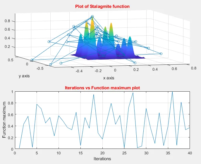
Plots for the above code:
Command window:
Study 2: Statistical behavior with upper and lower bounds
clear all
close all
clc

tiledlayout(2,1)
num_spaces = 40;

%Defining our search space
x = linspace(0,0.6,150);
y = linspace(0,0.6,150);

%Creating a 2D mesh
[xx yy] = meshgrid(x,y);

%Evaluating the stalagmite function
for i = 1:length(xx)
    for j = 1:length(yy)
        input_vector(1) = xx(i,j);
        input_vector(2) = yy(i,j);
        f(i,j) = stalagmite(input_vector);
    end
end

%Using ga() synatx with suitable arguments
tic
for i = 1:num_spaces
    [inputs,fout(i)] = ga(@stalagmite,2,[],[],[],[],[0;0],[0.4;0.4])
    xoutput(i) = inputs(1);
    youtput(i) = inputs(2);
end
studytime = toc

%plotting the meshgrid
nexttile
surfc(xx,yy,-f)
title('Plot of Stalagmite function','color','r')
xlabel('x axis')
ylabel('y axis')
shading interp
hold on
plot3(xoutput,youtput,-fout,'marker','o')
%plotting the F maximum vs no. of iterations
nexttile
plot(-fout)
title('Iterations vs Function maximum plot','color','r')
xlabel('Iterations')
ylabel('Function maximum')
axis([0 30 0.8 1.05])
grid on
ga() syntax for the above code:
[x,fval] = ga(fun,nvars,A,b,Aeq,beq,lb,ub) defines a set of lower and upper bounds on the design variables, x, so that a solution is found in the range lb ≤ x ≤ ub. (Set Aeq=[] and beq=[] if no linear equalities exist). Also, for any previous input arguments returns fval, the value of the fitness function at x.
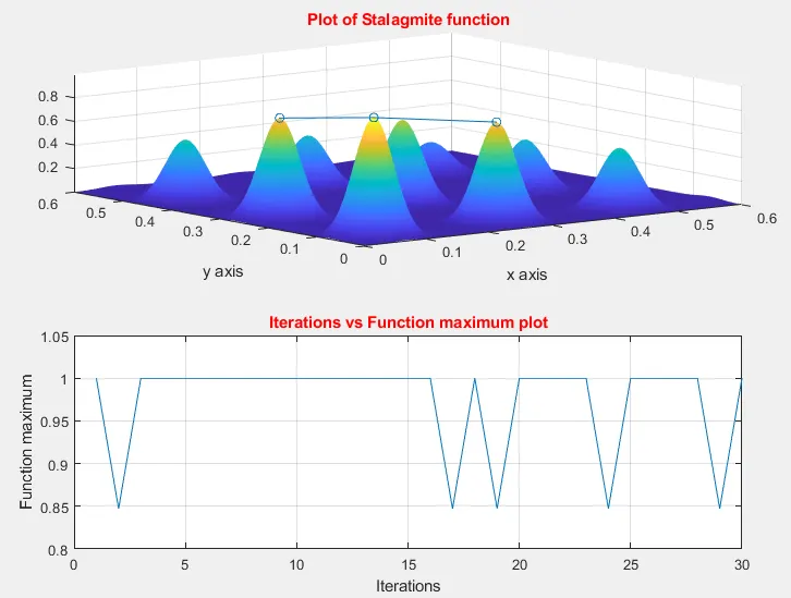
Plots for the above code:
Command window:
Study 3: Statistical behavior with upper and lower bounds in addition to specifying the bounds
clear all
close all
clc

tiledlayout(2,1)
num_spaces = 40;

%Defining our search space
x = linspace(0,0.6,150);
y = linspace(0,0.6,150);

%Creating a 2D mesh
[xx yy] = meshgrid(x,y);

options = optimoptions('ga');
options = optimoptions(options,'PopulationSize',200);

%Evaluating the stalagmite function
for i = 1:length(xx)
    for j = 1:length(yy)
        input_vector(1) = xx(i,j);
        input_vector(2) = yy(i,j);
        f(i,j) = stalagmite(input_vector);
    end
end

%Using ga() synatx with suitable arguments
tic
for i = 1:num_spaces
    [inputs,fout(i)] = ga(@stalagmite,2,[],[],[],[],[0;0],[0.5;0.5],[],[],options)
    xoutput(i) = inputs(1);
    youtput(i) = inputs(2);
end
studytime = toc

%plotting the meshgrid
nexttile
surfc(xx,yy,-f)
title('Plot of Stalagmite function','color','r')
xlabel('x axis')
ylabel('y axis')
shading interp
hold on
plot3(xoutput,youtput,-fout,'marker','o')
%plotting the F maximum vs no. of iterations
nexttile
plot(-fout)
title('Iterations vs Function maximum plot','color','r')
xlabel('Iterations')
ylabel('Function maximum')
axis([0 30 0.9999996 0.9999999])
grid on
Syntax for the above code:
ga():
[x,fval] = ga(fun,nvars,A,b,[],[],lb,ub,nonlcon,IntCon,options) defines a set of lower and upper bounds on the design variables, x, so that a solution is found in the range lb ≤ x ≤ ub. (Set Aeq=[] and beq=[] if no linear equalities exist). The syntax requires that the variables listed in IntCon take integer values. Also, for any previous input arguments returns fval, the value of the fitness function at x. The syntax minimizes with the default optimization parameters replaced by values in options. (Set nonlcon=[] if no nonlinear constraints exist.) Create options using optimoptions.
optimoptions():
options = optimoptions(SolverName) returns a set of default options for the SolverName solver. Here, solvername is 'ga'.
options = optimoptions(SolverName,Name,Value) returns options with specified parameters set using one or more name-value pair arguments.
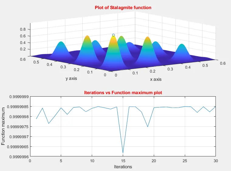
Plots for the above code:
Command window:
No such major errors were encountered while coding.
CONCLUSION:
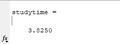
Study 1: The result shows, maxima vary over the large size of the interval, providing a vague idea of global maxima. Through the particular value of global maxima can't be determined but by observation, it can be figured that the value of global maximum lies between the interval [0,1]. Study time for this study was the least of all the three i.e., 3.8250 seconds.
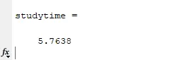
Study 2: The results shows, after providing the boundary limits the variation in the optimum values have reduced. From the plot, it can be inferred that the global maxima lie in the range [0.85,1]. The study time for this study was 5.7638 seconds.
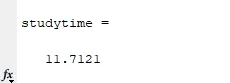
Study 3: By increasing the population size and incorporating founded inputs, we have more probability of determining the global maxima. The study time for this study was 11.7121 seconds.
REFERENCES: