Solving second order ODEs

AIM: To solve second order Ordinary Differential Equations.

Stepwise explanation of the code:

• All the geometric properties of the pendulum are defined i.e., b,g,m,l.
• Initial angular displacement and angular velocity are defined as a column matrix.
• Separate ode function in a separate MATLAB program which takes the input as (t,theta,b,g,l,m) and gives the output as [t,results].
• Results variable is the matrix having two columns, the first column for the angular displacement and the second column for the angular velocity.
• Then, the fixed end, the rod of the pendulum, and the bob is plotted using the plot() syntax inside the for loop.
• Later, for each iteration, the frames are stored in the variable M().
• Finally, each frame are stitched together to the final movie using movie() syntax.

Program code:

%solving the second order differential equation
clear all
close all
clc

% All units in the SI system
b = 0.05;
g = 9.81
l = 1;
m = 1;

%initial conditions
theta_r = [0;3];

%time points
t_span = linspace(0,20,300);

%calling the ODE function
[t,results] = ode45(@(t,theta) ode_funct(t,theta,b,g,l,m), t_span, theta_r);
%hold on
%plot(t,results(:,1))
%plot(t,results(:,2))
%ylabel('angular displacement')
%xlabel('time')

ct = 1;

for i=1:length(t_span)
    
    x0 = 0;%fixed end of the pendulum
    y0 = 0;
    
    x1 = l*sin(results(i,1));%position of the bob for the time value
    y1 = -l*cos(results(i,1));
    
    grid on
    plot([-0.5 0.5],[0 0],'linewidth',3,'color','black');%plotting the fixed end
    hold on
    
    plot([x0 x1],[y0 y1],'linewidth',3);%plotting the pendulum rod
    plot(x1,y1,'marker','o','markersize',15,'markerfacecolor','b')%plotting the bob
    hold off
    axis([-2 2 -2 2])
    pause(0.001);
    title('Simple Pendulum');
    M(ct) = getframe(gcf);
    ct = ct+1;
end

 %to create a movie
 movie(M)
 videofile = VideoWriter('pendulum.avi','Uncompressed AVI');
 open(videofile)
 writeVideo(videofile,M)
 close(videofile)

ode_funct code:

function [dtheta_dt] = ode_funct(t,theta,b,g,l,m)

theta1 = theta(1)
theta2 = theta(2)
dtheta1_dt = theta2;
dtheta2_dt = -(b/m)*theta2-(g/l)*sin(theta1);
[dtheta_dt] = [dtheta1_dt;dtheta2_dt];

end

OUTPUT:

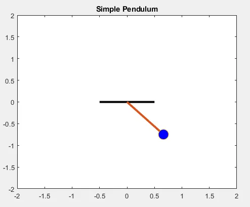
The link for the animation of the full video is given below:

https://youtu.be/_Or4z_iGWwM

CONCLUSION:

The animation of the simple pendulum can be done using MATLAB by stitching the frames together. The pendulum's geometric properties can be changed to get different animation of the simple pendulum.