Air standard Cycle

AIM: To write a MATLAB code that solves an Otto cycle and calculates its thermal efficiency.

THEORY: An Otto cycle is an idealized thermodynamic cycle that describes the functioning of a typical spark ignition piston engine. It is the thermodynamic cycle most commonly found in automobile engines.

The processes are described by:

• Process 0–1: A mass of air is drawn into a piston/cylinder arrangement at constant pressure.
• Process 1–2: It is an adiabatic (isentropic) compression of the charge as the piston moves from bottom dead center (BDC) to the top dead center (TDC).
• Process 2–3: It is a constant-volume heat transfer to the working gas from an external source while the piston is at the top dead center. This process is intended to represent the ignition of the fuel-air mixture and the subsequent rapid burning.
• Process 3–4: It is an adiabatic (isentropic) expansion (power stroke).
• Process 4–1: Completes the cycle by a constant-volume process in which heat is rejected from the air while the piston is at the bottom dead center.
• Process 1–0: The mass of air is released to the atmosphere in a constant pressure process.

Characteristics of the process:

• Process 1-2: Isentropic Compression
• Process 2-3: Constant Volume heat addition
• Process 3-4: Isentropic Expansion
• Process 4-1: Constant Volume heat rejection

FORMULAE:

Gas equation,

• pV = nRT

For isentropic compression and expansion,

• pV^κ = constant

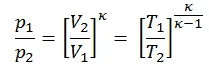
P, V, T relations,

• 

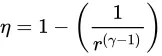
Thermal efficiency,

• 

Swept volume,

The swept volume is the volume of air displaced by the piston's diameter in one full stroke from BDC to TDC.

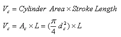
Clearance Volume,

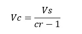
The change of volume with respect to crank angle,

Here,

a = crankpin radius

rc = compression ratio

`theta`= Crank angle

Explanations:

• The input values are allocated.
• The state variables like Pressure, Volume and Temperature are found out using the above formulas for states 2,3, and 4. t3 is given.
• For the isentropic compression and expansion curve, there is a relation given between the Volume of the cylinder and crank angle.
• Function engine_kinematics is called to calculate volume along with the change in crank angle for compression stroke and expansion stroke.
• After all state parameters are found out, the thermal efficiency of the engine is calculated.
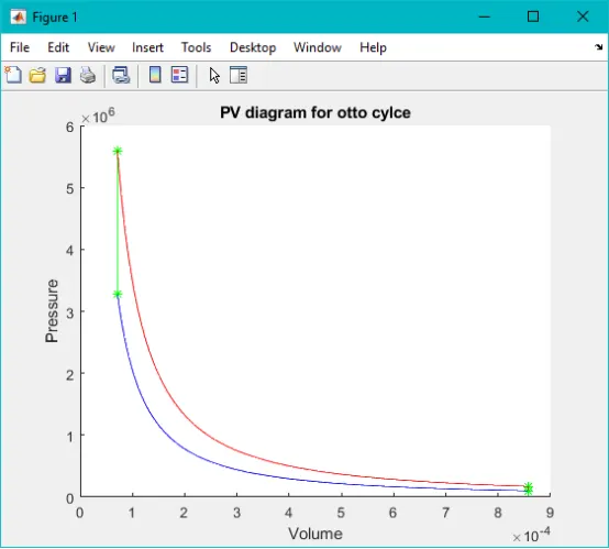
• Finally, PV diagram is plotted for the above parameters.

Main code:

%program to plot PV diagram for Otto cycle and calculate the thermal
%efficiency
clear all
close all
clc

%inputs
gamma = 1.4;
t3 = 2300;
p1 = 101325;
t1 = 500;

%engine geometric parameters
bore = 0.1;
stroke = 0.1;
con_rod = 0.15;
cr = 12;

%calculating the swept volume and the clearance volume
v_swept = pi*(bore/2)^2*stroke;
v_clearance = v_swept/(cr-1);
v1 = v_swept + v_clearance;
v2 = v_clearance;

constant_c = p1*v1^gamma;
v_compression = engine_kinematics(bore,stroke,con_rod,cr,180,360);
p_compression = constant_c./v_compression.^gamma;

%State point 2
p2 = p1*(v1/v2)^gamma;
t2 = t1*(v1/v2)^(gamma-1);


%state point 3
v3 = v2;
p3 = p2*t3/t2;

constant_c = p3*v3^gamma;
v_expansion = engine_kinematics(bore,stroke,con_rod,cr,0,180);
p_expansion = constant_c./v_expansion.^gamma;

%state variables at state point 4
v4 = v1;
p4 = p3*(v3/v4)^gamma;
t4 = t3*(v3/v4)^(gamma-1);

%thermal efficiency of the engine
t_efficiency = 1-(1/cr^(gamma-1))

hold on
plot([v1 v2 v3 v4],[p1 p2 p3 p4],'*','color','g')
plot(v_compression,p_compression,'color','b')
plot([v2 v3],[p2 p3],'color','g')
plot([v_expansion v1],[p_expansion p1],'color','r')
title('PV diagram for otto cylce')
xlabel('Volume')
ylabel('Pressure')

Function code:

function [v] = engine_kinematics(bore,stroke,con_rod,cr,start_angle,end_angle)

a = stroke/2;
R = cr/a;
theta = linspace(start_angle, end_angle, 180)

v_s = (pi/4)*bore^2*stroke;
v_c = v_s/(cr-1);

term1 = 0.5*(cr-1);
term2 = R+1-cosd(theta);
term3 = (R^2-sind(theta).^2).^0.5;

v = (1+term1*(term2-term3))*v_c;

end

Output results:

Different colors represent respective states in the Otto cycle,

Blue - Compression

Red - Expansion

Green - Constant volume processes

Thermal Efficiency:

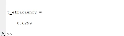
Hence, the thermal efficiency for the above plot is found out to be 62.99%.

CONCLUSION:

By varying different parameters of the engine, respective PV plots can be obtained. Also, plots for the Diesel cycle and the Dual cycle can be obtained by varying its characteristics equation.