Curve fitting

AIM: To fit a linear and cubic polynomial for the given Cp data. And to write a code to show splitwise method.

THEORY:

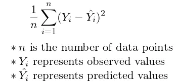
1. MSE(Mean Squared Error): It measures the average of the squares of the errors that is the average squared between the estimated values and the actual values. We take the mean of the individual squared error terms in order to calculate MSE. The general formula for MSE is given below,

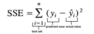
2. SSE(Sum of Squared Error): It measures the total deviation of the response values from the fit to the response values it is called as Sum of Squared Error. The general formula for SSE is given below,

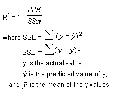
3. R-Square: It is a statistical measure that represents the proportion of the variance for a dependent variable that is explained by an independent variable or variables in a regression model. It is also known as the coefficient of determination. R-square values range from 0 to 1 and are commonly stated as percentages from 0 to 100%. In analysis, if the R-square value is 1, t is known as a perfect fit. The general formula for R-square is given below,

Explanation of the code:

• Firstly, the data is extracted into a variable called cp_data.
• Then the temperature values and cp values from the cp_data is stored in the variables temperature and cp.
• Using these temperatures and cp values, linear and cubic curve is fit.
• The curve is fitted using the polyfit() and polyval() syntax.
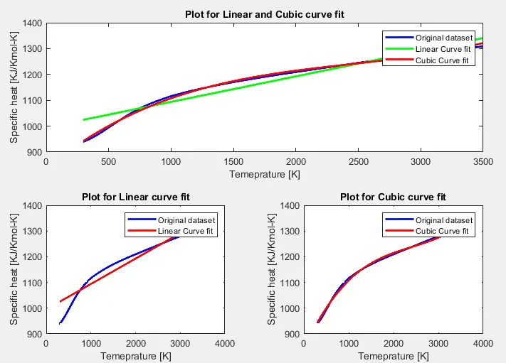
• Three plots are plotted with temperature vs specific heat as the axis parameters.

Program code to fit a linear and cubic polynomial for the Cp data:

clear all
close all
clc

tiledlayout(2,2);
%preparing the data
cp_data = load('tempcp_data');
temperature = cp_data(:,1);
cp = cp_data(:,2);

%linear curve fit cp = a*T+b
co_effs = polyfit(temperature,cp,1);
cp1 = polyval(co_effs,temperature);

%cubic curve fit cp = a*T^3+b*T^2+c*T+d
co_effs = polyfit(temperature,cp,3);
cp3 = polyval(co_effs,temperature);

%comparing linear curve fit with the original data
nexttile(3)
plot(temperature,cp,'linewidth',2,'color','b')
hold on
plot(temperature,cp1,'linewidth',2,'color','r')
xlabel('Temeprature [K]')
ylabel('Specific heat [KJ/Kmol-K]')
legend('Original dataset','Linear Curve fit')
title('Plot for Linear curve fit')

%comparing cubic curve fit with the original data
nexttile(4)
plot(temperature,cp,'linewidth',2,'color','b')
hold on
plot(temperature,cp3,'linewidth',2,'color','r')
xlabel('Temeprature [K]')
ylabel('Specific heat [KJ/Kmol-K]')
legend('Original dataset','Cubic Curve fit')
title('Plot for Cubic curve fit')


%comparing linear curve fit and cubic curve fit with the original data
nexttile(1,[1 2])
plot(temperature,cp,'linewidth',2,'color','b')
hold on
plot(temperature,cp1,'linewidth',2,'color','g')
plot(temperature,cp3,'linewidth',2,'color','r')
xlabel('Temeprature [K]')
ylabel('Specific heat [KJ/Kmol-K]')
legend('Original dataset','Linear Curve fit','Cubic Curve fit')
title('Plot for Linear and Cubic curve fit')

Plots for the above code:

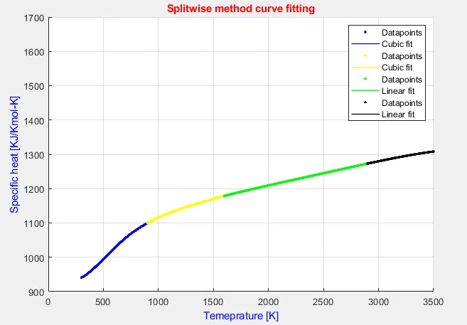
Explanation for the stepwise method:

• Firstly, the data is extracted into a variable called cp_data.
• Next, the 3200 values in the cp_data are split into 4 variables as mentioned in the code.
• Using the fit() syntax, the curves are fitted from the given data.
• Then plotting is done using the plot() syntax.
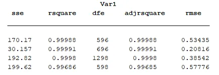
• The goodness of fit 'gof', that is returned from the function fit() is then stored in a table to display the values later on.
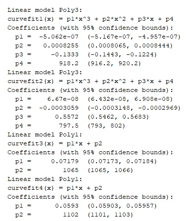
• Then, the mathematical models are displayed.

Program code for the stepwise regression method:

%curve fitting by stepwise regression method
clear all
close all
clc

cp_data = load('tempcp_data');
temperature = cp_data(:,1);
cp = cp_data(:,2);

%splitting the temperature and Cp data into 4 variables
temp1 = cp_data(1:600,1);
cp1 = cp_data(1:600,2);

temp2 = cp_data(601:1300,1);
cp2 = cp_data(601:1300,2);

temp3 = cp_data(1301:2600,1);
cp3 = cp_data(1301:2600,2);

temp4 = cp_data(2601:3200,1);
cp4 = cp_data(2601:3200,2);

hold on 
grid on

%plotting the data
[curvefit1,gof1] = fit(temp1,cp1,'poly3');
a = plot(curvefit1,temp1,cp1);
set(a,'linewidth',1,'color','b');

[curvefit2,gof2] = fit(temp2,cp2,'poly3');
b = plot(curvefit2,temp2,cp2);
set(b,'linewidth',1,'color','y');

[curvefit3,gof3] = fit(temp3,cp3,'poly1');
c = plot(curvefit3,temp3,cp3);
set(c,'linewidth',1,'color','g');

[curvefit4,gof4] = fit(temp4,cp4,'poly1');
d = plot(curvefit4,temp4,cp4);
set(d,'linewidth',1,'color','black');
axis([0 3500 900 1700]);

%Goodness Parameter's table
aTable = struct2table(gof1);
bTable = struct2table(gof2);
cTable = struct2table(gof3);
dTable = struct2table(gof4);
T = table([aTable;bTable;cTable;dTable]);
disp(T)

%plot labelling
legend('Datapoints','Cubic fit','Datapoints','Cubic fit','Datapoints','Linear fit','Datapoints','Linear fit');
xlabel('Temeprature [K]','color','b')
ylabel('Specific heat [KJ/Kmol-K]','color','b')
title('Splitwise method curve fitting','color','r');

%Displaying Mathematical model
disp(curvefit1);
disp(curvefit2);
disp(curvefit3);
disp(curvefit4);

Plots for the above code:

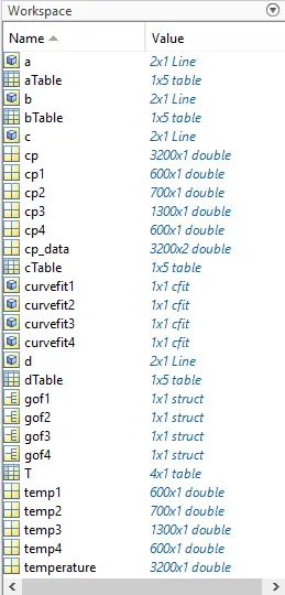
Command window:

Syntaxes:

• fit(): [fitobject,gof] = fit(x,y,fitType) creates the fit to the data in xand y with the model specified by fitType and returns goodness-of-fit statistics in the structure gof.
• polyfit(): p= polyfit(x,y,n) returns the coefficients for a polynomial p(x) of degree n that is the best fit (in a least-squares sense) for the data in y. The coefficients in p are in descending powers, and the length of p is n+1. p(x)=p1xn+p2xn−1+...+pnx+pn+1.
• ployval(): y= polyval(,x) evaluates the polynomial p at each point in x. The argument p is a vector of length n+1 whose elements are the coefficients (in descending powers) of an nth-degree polynomial: p(x)=p1xn+p2xn−1+...+pnx+pn+1.

No major errors were faced during coding.

REFERENCES:

https://projects.skill-lync.com/projects/Curve-Fitting-and-criterion-to-choose-best-fit-41860

https://in.mathworks.com/matlabcentral/answers/157183-polyfit-with-centering-and-scaling-values

CONCLUSION:

How to make a perfect fit: In order to make a perfect fit, we must consider error estimates as well. The perfect fit means, the curve should fit the original curve without showing any errors (such as scaling and centering errors) in that particular degree if the polynomial. A perfect fit can always be the best fit but the best fit cannot be a perfect fit. Hence, to calculate the best fit, we must increase the order or use splitwise method.

How to get the best fit: For this, the best way is to split the data into two or more data folds and do the curve fit.

What could be done to improve the cubic fit: We can use the splitwise regression method. In this method, in the above code, the data is split into four data folds.