Week 4.1 - Genetic Algorithm
Challenge:
- Write a code in MATLAB to optimise the stalagmite function and find the global maxima of the function.
- Clearly expalin the concept of genetic algorithm in your own words and also explain the syntax for ga in MATLAB in your report.
- Make sure that your code gives the same output, even if it is made to run several times.
- Plot graphs for all 3 studies and for F maximum vs no. of iterations. Title and axes labels are a must, legends could be shown if necessary.
Concept of Genetic Algorithm explained.
The main goal of using the Genetic Algorithm in MATLAB is to find the minimal values of a function. In a more general optic, Genetics Algorithms are used widely in optimizations of mathematical problems. Other uses can also be found in the fields of econimics, neutral network and image processing.
In our situation here, we will creating an optimisation process to find the best solution to a given problem. Although there are other optimisation techniques available from a mathematical point of view, like deterministic or stochastics algoritithms, we will be studying the Genetic Algorithm.
Advantages of GAs , from Tutorialpoints.com
GAs have various advantages which have made them immensely popular. These include −
-
Does not require any derivative information (which may not be available for many real-world problems).
-
Is faster and more efficient as compared to the traditional methods.
-
Has very good parallel capabilities.
-
Optimizes both continuous and discrete functions and also multi-objective problems.
-
Provides a list of “good” solutions and not just a single solution.
-
Always gets an answer to the problem, which gets better over the time.
-
Useful when the search space is very large and there are a large number of parameters involved.
Limitations of GAs
Like any technique, GAs also suffer from a few limitations. These include −
-
GAs are not suited for all problems, especially problems which are simple and for which derivative information is available.
-
Fitness value is calculated repeatedly which might be computationally expensive for some problems.
-
Being stochastic, there are no guarantees on the optimality or the quality of the solution.
-
If not implemented properly, the GA may not converge to the optimal solution.
Here is more precise definition found on wikipedia:
"In computer science and operations research, a genetic algorithm (GA) is a metaheuristic inspired by the process of natural selection that belongs to the larger class of evolutionary algorithms (EA). Genetic algorithms are commonly used to generate high-quality solutions to optimization and search problems by relying on biologically inspired operators such as mutation, crossover and selection."
A typical genetic algorithm requires:
- a genetic representation of the solution domain,
- a fitness function to evaluate the solution domain.
A population of different solution is generate in form of an array. Each solution will have randomly generated values and each solution of the population will be the size of array, making the processing easier. Then using the fitness function, each indicidual solution will be tested for fitness and the process will go again with the most fit solution. A new generation of population will be generated again, using genetics operators, crossover and mutation, and tested for fitness and so on.
"Commonly, the algorithm terminates when either a maximum number of generations has been produced, or a satisfactory fitness level has been reached for the population."
Explain the syntax for ga in MATLAB in your report.
The built in Genetix algorithm in MATLAB has a lot of different possible configurations. I will explain here the ones we are using in this program. Below an overview of all the different possiblities, I got from MATLAB help documentation.
Syntax
The program is calling the 'ag' command in our primary attempt to find the minimum value of the stalagmite function. This is the simplest way to use this command. The 'ga' function in this case will need to be given 2 inputs arguments, 'x' and 'nvars'. We combine that with requesting for output, 'x' for the input variables in the function we are optimizing and 'fval' for the minimum function value.
[inputs,fval]=ga(@stalagmite,2)
We want to obtain the different results, 'inputs' and 'fval'. The variable named 'fval' is the minimum value of the function that the 'ga' command will give us. The other variable, 'inputs', will be the 'x' and 'y' values at which the function is giving us that minimum value. On the input side, we are giving the arguments, firstly the target function, 'stalagmite' and secondly the number of variables, 2 in this case.
x = ga(fun,nvars,A,b,Aeq,beq,lb,ub)x, so that a solution is found in the range lb ≤ x ≤ ub. (Set Aeq=[] and beq=[] if no linear equalities exist.)
In this particular program, on the second instance of using the command 'ga', we are specifing additonal arguments, 'lb' and 'ub'. They stand for Lower Bound and Upper Bound. Because we know the result we are looking for in the function being processed dosen't good results for inputs smaller than 0 or larger than 1, we want to set boundaries. This will make the processing of our algorithm more focussed and save processing time and power.
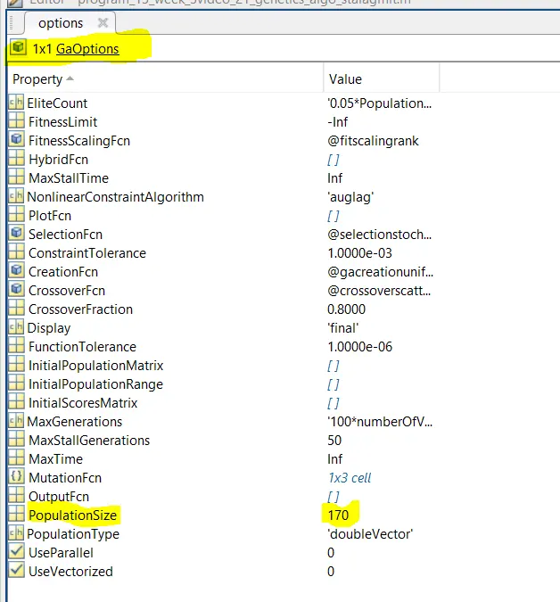
In the third instance of using the command 'ga', we are specifing additonal arguments, using the 'options' argument. There are multitiude of possible options we could specify for the function 'ga'. Below is attached a screen shot of the option registery in my program. I higlighted the one in particular we are using, 'PopulationSize'. We see that the 'ga' function of MATLAB looks really powerful and we only scratching the surface.
x = ga(fun,nvars,A,b,Aeq,beq,lb,ub,nonlcon,options)options. (Set nonlcon=[] if no nonlinear constraints exist.) Create options using optimoptions.
Main program explaination:
%This program will experiment with genetic algorithm using MATLAB
%Written by Dave Levesque following the video 21 and 22 example

%program initalization
clear all % clear all variable from previous programs or previous executions
close all % close all windows, graphics and tables previously generated by mathlab
clc % Clear command window

%Preparing the data

%defining our search space
x = linspace(0,0.6,150);
y = linspace(0,0.6,150);

% number of time the genetic algo to run
case_num = 50;
%linking stalagmite function
%F2=get_stalagmite
%Creating a 2 dimension mesh
[xx,yy]= meshgrid(x,y);

%evaluating the stalagmite function
for i = 1:length(xx);
    for j = 1:length(yy);
        input_vector(1)=xx(i,j);
        input_vector(2)=yy(i,j);
        F(i,j) = stalagmite(input_vector);
    end
end

% plotting the graphic area
figure(1)
surfc(xx,yy,F)
%axis identification
xlabel('X value')
ylabel('Y value')

%removing the 3D grid lines
shading interp

%Results without optimization
%Applying the genetics algo
[inputs,fval]=ga(@stalagmite,2)

%Optimization Studies

% Study #1 - without boundaries
%timer on
tic
for i =1 : case_num
  [inputs,fval_opt(i)]=ga(@stalagmite,2);
  xopt(i)=inputs(1);
  yopt(i)=inputs(2);
end
%timer off
study_1_time = toc

figure(2)
subplot(2,1,1)
hold on
surfc(x,y,F)
shading interp
plot3(xopt,yopt,fval_opt,'marker','o','markersize',5,'markerfacecolor','r')
title('Unbounded inputs')
subplot(2,1,2)
plot(fval_opt)
xlabel('iterations')
ylabel('Function minimun')

% Study #2 - with defined boundaries
%timer on
tic
for i =1 : case_num
 [inputs,fval_opt(i)]=ga(@stalagmite,2,[],[],[],[],[0,0],[1,1]);
  xopt(i)=inputs(1);
  yopt(i)=inputs(2);
end
%timer off
study_2_time = toc

figure(3)
subplot(2,1,1)
hold on
surfc(x,y,F)
shading interp
plot3(xopt,yopt,fval_opt,'marker','o','markersize',5,'markerfacecolor','r')
title('Unbounded inputs')
subplot(2,1,2)
plot(fval_opt)
xlabel('iterations')
ylabel('Function minimun')


% Study #3 - increasing the number of 'ga' iterations
options = optimoptions('ga')
options = optimoptions(options,'PopulationSize',170);
tic
for i =1 : case_num
 [inputs,fval_opt(i)]=ga(@stalagmite,2,[],[],[],[],[0,0],[1,1],[],[],options);
  xopt(i)=inputs(1);
  yopt(i)=inputs(2);
end
%timer off
study_3_time = toc

figure(4)
subplot(2,1,1)
hold on
surfc(x,y,F)
shading interp
plot3(xopt,yopt,fval_opt,'marker','o','markersize',5,'markerfacecolor','r')
title('Unbounded inputs')
subplot(2,1,2)
plot(fval_opt)
xlabel('iterations')
ylabel('Function minimun')

%The end
Program initialization:
In order to start on a clean slate, the first funtions of my code are the followings, clear all, close all and clc.
clear all : clear all variable from previous programs or previous executions
close all : close all windows, graphics and tables previously generated by matlab
clc : clear command window
Preparing the data: The first step is to organize the starting variables and data. Here, the search space is the range of values, for X and Y that will be evaluated. The variable 'case_num' will be used later by the genetics algorithm, for the number of iterations to be run. Next, we are creating a mesh, for x and y.
"[ returns 2-D grid coordinates based on the coordinates contained in vectors X,Y] = meshgrid(x,y)x and y. X is a matrix where each row is a copy of x, and Y is a matrix where each column is a copy of y. The grid represented by the coordinates X and Y has length(y) rows and length(x) columns."
%defining our search space
x = linspace(0,0.6,150);
y = linspace(0,0.6,150);
% number of time the genetic algo to run
case_num = 50;
%Creating a 2 dimension mesh
[xx,yy]= meshgrid(x,y);
Main Program - First attempt without optimization :
We are now evaluating the result of the function 'stalagmite' in all its iterations possible. It is running all the possible X and Y, as a double loop, and storing the results in the variable 'F'. This variable is a large array compromising all the results, 150 x 150 times.
%evaluating the stalagmite function
for i = 1:length(xx);
for j = 1:length(yy);
input_vector(1)=xx(i,j);
input_vector(2)=yy(i,j);
F(i,j) = stalagmite(input_vector);
end
end
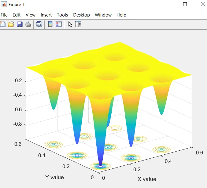
After, we are plotting this first results on a 3D plot. The command 'surfc' is use to define the area of the plot, as a surface. We are using the values in the vector, xx and yy and for the third dimension, the third axis z, the value of the funtion is used.
% plotting the graphic area
figure(1)
surfc(xx,yy,F)
%axis identification
xlabel('X value')
ylabel('Y value')
%removing the 3D grid lines
shading interp
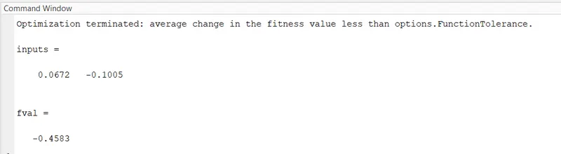
As a final step, we are applying the genetic algorithm to attemp to get the minimal value of the function. Because there is no optimization, we don't consistently get the same results. We have a good estimate, of the x and y values that are giving us that aproximation. We can see it on the 3D plot.
%Results without optimization
%Applying the genetics algo
[inputs,fval]=ga(@stalagmite,2)
Figure 1
Main Program - Second attempt with optimization Study #1 :
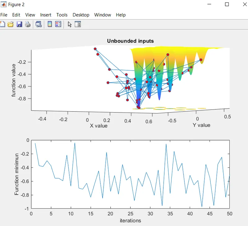
We are now plotting the different results of the genetic algorithm in a more complex plot. That is leading us to see that we are evaluating some results for some values that are outside the range, so not very useful. Eventhough we are beginning with the X and Y values between 0 and 0.6, the random effect of the genetic algorithm ended up getting values all over the place. We are using the command 'tic' and 'toc' for the first time. These are used to calculate the time is takes to exucutes the code in bewteen, and we are storing the value in second, in a variable.
figure(2)
subplot(2,1,1)
hold on
surfc(x,y,F)
shading interp
plot3(xopt,yopt,fval_opt,'marker','o','markersize',5,'markerfacecolor','r')
title('Unbounded inputs')
xlabel('X value')
ylabel('Y value')
ylabel('function value')
subplot(2,1,2)
plot(fval_opt)
xlabel('iterations')
ylabel('Function minimun')
Figure 2
Main Program - Third attempt with optimization Study #2 :
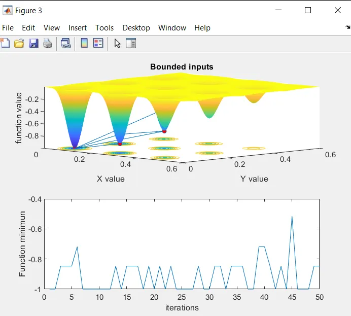
We are now going to redo the same thing, but this time with boundaries. To achieve this, we are using an extra argument in the 'ga' command. This will run the algoirthm using values that are within the range specified. The values of x and y, will be between 0 and 1.
for i =1 : case_num
[inputs,fval_opt(i)]=ga(@stalagmite,2,[],[],[],[],[0,0],[1,1]);
xopt(i)=inputs(1);
yopt(i)=inputs(2);
end
%timer off
study_2_time = toc
figure(3)
subplot(2,1,1)
hold on
surfc(x,y,F)
shading interp
plot3(xopt,yopt,fval_opt,'marker','o','markersize',5,'markerfacecolor','r')
title('Bounded inputs')
xlabel('X value')
ylabel('Y value')
ylabel('function value')
subplot(2,1,2)
plot(fval_opt)
xlabel('iterations')
ylabel('Function minimun')
Figure 3
Main Program - Fourth attempt with optimization Study #3 :
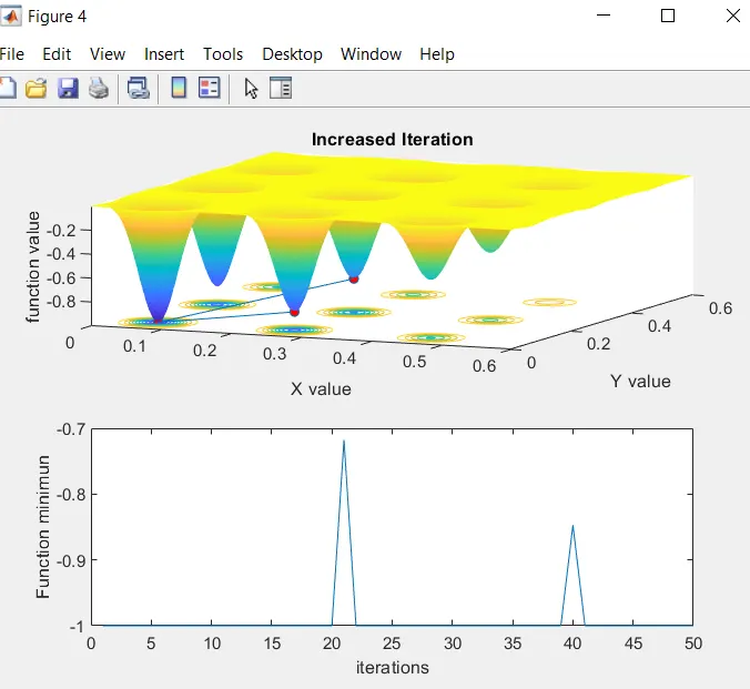
Due to the nature of the genetics algorithm, we have still a large number of possible fuction values. This could be due to our first initial population being too small. We will try again the genetic alogorithm with a larger number of iteration. We will specify an extra optional argument, 'PopulationSize'. See the section AG syntaxe for more details.
% Study #3 - increasing the number of 'ga' iterations
options = optimoptions('ga')
options = optimoptions(options,'PopulationSize',170);
tic
for i =1 : case_num
[inputs,fval_opt(i)]=ga(@stalagmite,2,[],[],[],[],[0,0],[1,1],[],[],options);
xopt(i)=inputs(1);
yopt(i)=inputs(2);
end
%timer off
study_3_time = toc
figure(4)
subplot(2,1,1)
hold on
surfc(x,y,F)
shading interp
plot3(xopt,yopt,fval_opt,'marker','o','markersize',5,'markerfacecolor','r')
title('Increased Iteration')
xlabel('X value')
ylabel('Y value')
zlabel('function value')
subplot(2,1,2)
plot(fval_opt)
xlabel('iterations')
ylabel('Function minimun')
Figure 4
Function stalagmite
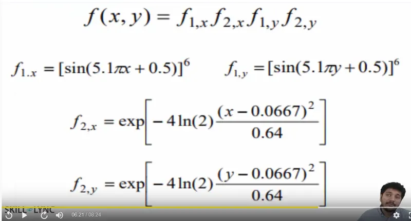
Based on the equation of the stalagmite, I created a sub-program to process it.
function [F]= stalagmite(input_vector)
%input assignment
x=input_vector(1);
y=input_vector(2);

%The function is divided in 4 terms
f1x=(sin((5.1*pi)*x + 0.5)).^6;
f1y=(sin((5.1*pi)*y + 0.5)).^6;
f2x=exp(((-4*log(2)).*(((x-0.0667).^2)/0.64)));
f2y=exp(((-4*log(2)).*(((y-0.0667).^2)/0.64)));

% f1x= (sin((5.1*pi).*input_vector(1)+0.5)).^6;
% f1y= (sin((5.1*pi).*input_vector(2)+0.5)).^6;
% f2x= exp((((input_vector(1)-0.0667).^2)/0.64).*(-4*log(2)));
% f2y= exp((((input_vector(2)-0.0667).^2)/0.64).*(-4*log(2)));


% function terms assembled in the final fucntion F
 F1=f1x*f1y*f2x*f2y;
 F=-F1;

%F=f1x*f1y*f2x*f2y;
end
Errors faced while programing:
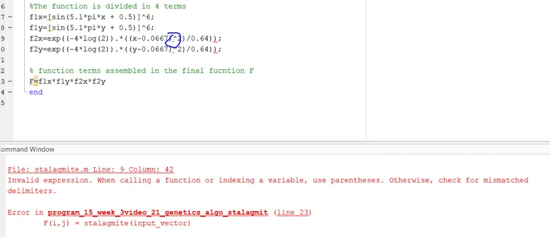
Error 1:Invalid expression. When calling a function or indexing a variable, use parentheses. Otherwise, check for mismatched
delimiters.
Cause: MATLAB is unable to process that line of operations. It could be because of a missing '.' or parenthese. The '.' is sometimes required in MATLAB to indicate element-wise as opposed to array operations. The dot was missing in between elements to be multiplied.
Corrective: Once the function spelled and typed in correctly, it was recongnized by MATLAB and the error was gone.
References:
MATLAB help documentation
https://skill-lync.com/knowledgebase/genetic-algorithm-explained
https://en.wikipedia.org/wiki/Genetic_algorithm
https://www.tutorialspoint.com/genetic_algorithms/genetic_algorithms_introduction.htm