Week 3 - Solving second order ODEs

Challenge:

The objective is to write a program that solves the following ODE. This ODE represents the equation of motion of a simple pendulum with damping

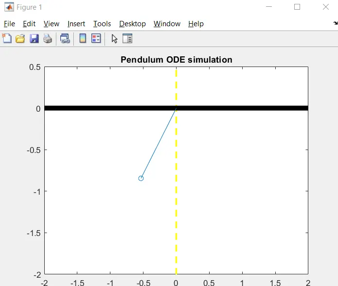
Part 1: Write a program in Matlab\Octave that will simulate the pendulum motion, just like the one shown in the start of this challenge.

Part 2: Create an animation of the position of the pendulum as a function of time.

Part 1 code, explainations and reccord of errors and corrections.

By the mean of the command "Insert CODE Sample", here is the code I wrote in MATHLAB

Main Code:

%This program will solve a second order ODE
%Written by Dave Levesque following the video 16 example

%program initalization 
clear all % clear all variable from previous programs or previous executions
close all % close all windows, graphics and tables previously generated by mathlab
clc % Clear command window

%Declaration of variables

b=0.05;  %dampening coeficient
g=9.81; % gravity in m/s2
l=1;    %length of the pendulum in meter
m=1;  % mass of the pendulum ball in kg
rotation_center =[0 0] %coordinate of the fixed rotation center.
pendulum_swing_radius = l %same as the length, 'l' defined ealier
ct = 1;%counter


%Initial conditions

theata_0=[0;3]; %at time 0, the starting angle is 0 and velocity 3
%for angular displacement=0,angular velocity=3 rad/sec at time t=0

%time points
t_span = linspace(0,20,100); %For time span 0 to 20, in 100 increments

%Solve ODE by calling the function 'ode_func'
[t,results]=ode45(@(t,theata) ode_func(t,theata,b,g,l,m),t_span, theata_0);

%Calculating and plotting the position of pendulum of each time frame.
result_row_n=1 % variable used to update the row number when reading from array.

for i=1:length(t_span) %Loop1 - excuted for each increment of theta 1

    pend_X=-l*sin(results(result_row_n,1))
    pend_y=-1*cos(results(result_row_n,1))
    result_row_n=result_row_n+1
    
    %Plotting the pendulum movement
    plot(pend_X, pend_y,'marker','o')
    
    %graphic area additions
    title('Pendulum ODE simulation')
    axis([-2 2 -2 0.5])
    % printing a dashed line, vertical along the y axis
    line([0 0],[-2 0.5],'color','y', 'linestyle', '--','linewidth', 2) 
    % tracing the top line, wide and black
    line([-2 2],[0 0],'color','k', 'linewidth', 6)
    % tracing the pendulum string
    line([0 pend_X],[0 pend_y])
    %pause (1) %pause 1 second.
    
    % Get Current Figure window
     M(ct)= getframe(gcf);
     %incrementing the counter
     ct=ct+1;
end  % end of the loop

%Generating the movie file 

movie(M)
videofile = VideoWriter('Pendulum_ODE_simulation.avi','Uncompressed AVI');
open(videofile)
writeVideo(videofile, M)
close(videofile)

%plotting results curves in figure 1 window
plot(t, results(:,1))
hold on
plot(t, results(:,2))
xlabel('time')
ylabel('Plot')
pause (1) %pause 1 second.


%The end

Program initialization:

In order to start on a clean slate, the first funtions of my code are the followings, clear all, close all and clc.

clear all : clear all variable from previous programs or previous executions
close all : close all windows, graphics and tables previously generated by mathlab
clc : clear command window

Declaration of variables:

The variables and their values are declared in the next section of the program as follow:

Inputs - List of the variables and values the program will use when running from the beginning

Initial conditions and associated values, and their respective units.

b=0.05; %dampening coeficient
g=9.81; % gravity in m/s2
l=1; %length of the pendulum in meter
m=1; % mass of the pendulum ball in kg
rotation_center =[0 0] %coordinate of the fixed rotation center.
pendulum_swing_radius = l %same as the length, 'l' defined ealier
ct = 1; %counter

Initial conditions of the pendulum are defined in the challenge statement. The initial displacement angle of the pendulum is 0 rad, the angular velocity is 3 rad/sec at time =0.

theata_0=[0;3]; %at time 0, the starting angle is 0 and velocity 3

The time points are set like this; for a time frame going from 0 sec to 20 sec, we will have 100 increments of time.

t_span = linspace(0,20,100);

Main code: solving the ODE

The ODE is solved by the mean of calling the custom made function 'ode_func' and also the existing MATHLAB funtion 'ode45'.

This line of code will generate the values we need, the displacement and velocity for each time increment. The results, is to be store in the array 't' for the time and 'results' , in two colunm for the displacement and velocity. The function is recongnizing the previously defined variables, such as, 'theata', 'b','g', ' l ' , 'm' and 't_span'.

[t,results]=ode45(@(t,theata) ode_func(t,theata,b,g,l,m),t_span, theata_0);

Calculating and plotting the position of pendulum of each time frame.

The additiona varialbe 'result_row_n' will be used later to keep track of the row number to get the data, in the 'results' arry, in the loop.

result_row_n=1

The loop is now being programmed as follow. It will be executed for each increment of time specified in 't_span' at the beginning of the program.

for i=1:length(t_span)

The x and y coordinated of the ball of the pendulum are now calculated using trigonometry. Beginning from the initial position of the ball, x=0 and y = -1. The angle, in rad, in pulled from the first colunm of the array 'results'. The row number is then incremented by 1 for the next time the loop will run.

pend_X=-l*sin(results(result_row_n,1))
pend_y=-1*cos(results(result_row_n,1))
result_row_n=result_row_n+1

Plotting the pendulum movement is achieved by the line of code below. Here the plot command is used to plot a 'marker' instead of a curve or a line. The argument 'o' is the shape of the marker to be used.

plot(pend_X, pend_y,'marker','o')

In order to generate a graphinc that looks great and provide a good visual presentation, I am adding the following lines for each figure. There is the graphic title, the axis definition, the fixed line on top where the pendulum is hanging from, a line representing the y axis and a line representing the string of the pendulum.

%graphic area additions
title('Pendulum ODE simulation')
axis([-2 2 -2 0.5])
% printing a dashed line, vertical along the y axis
line([0 0],[-2 0.5],'color','y', 'linestyle', '--','linewidth', 2)
% tracing the top line, wide and black
line([-2 2],[0 0],'color','k', 'linewidth', 6)
% tracing the pendulum string
line([0 pend_X],[0 pend_y])

The lines of code below are use to store the figure number. This will be required later when generating the movie file from the figures.

% Get Current Figure window
M(ct)= getframe(gcf);
%incrementing the counter
ct=ct+1;
end% end of the loop.

Generating the movie file:

The command movie(M) is used here. It plays the movie frames in array M once. In this case, the values in the array M are generate from the main loop above, representing the frame numbers, the figure number.

movie(M)

We are creating then the variable videofile that will be equal to the result of the function VideoWriter. When calling the function, we specify the movie file type and name and format.

videofile = VideoWriter('Pendulum_ODE_simulation.avi','Uncompressed AVI');

Now the program will open our video file, write the frames as per array M, and close it.
open(videofile)
writeVideo(videofile, M)
close(videofile)

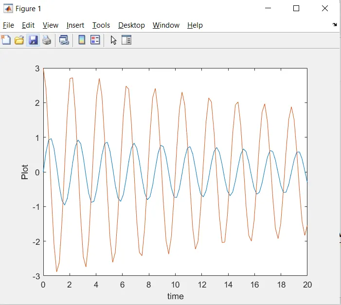
Plotting results curves in figure 1 window.

This is done using the command plot. it is plotting a first curce, displacement and a second curve, velocity. It is using the time on the x axis and the the values found in the array ' results' for the y axis. This figure can be seen below.
plot(t, results(:,1))
hold on
plot(t, results(:,2))
xlabel('time')
ylabel('Plot')
pause (1) %pause 1 second.

Part 1b: plotting the graph of the curve.

As I learned in the video, here is a graphic representation of the curves displacement vs time, and velocity vs time. We can clearly see that the displacement begins at 0 and then oscillate between 1 and -1. We can also see really well the velocity, decreasing and increasing, representing the acceleration and decelaration. The displacement is the blue curve, and the velocity is in red.

Part 1c: Function 'ode_func'

To accomplish the calculation of the displacement and velocity, the custom function have been created, called 'ode_func'. This helps us keeping the program more organized, by keeping this calculation in a seperate block. Another advantage is that we can re use that function, that block, into another project later, by simply recalling the funtion.

By the mean of the command "Insert CODE Sample", here is the code I wrote in MATHLAB, here the code for the function.

Custon made function:

function [dtheata_dt]= ode_func(t,theata,b,g,l,m)

theata1=theata(1)
theata2=theata(2)
dtheata1_dt=theata2
dtheata2_dt= -(b/m)*theata2 - (g/1)*sin(theata1)
dtheata_dt= [dtheata1_dt; dtheata2_dt]

end

Errors faced while programming.

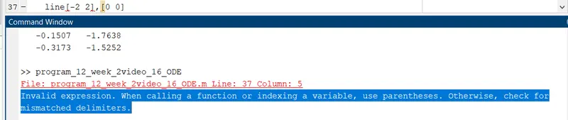
Error 1:Invalid expression. When calling a function or indexing a variable, use parentheses. Otherwise, check for
mismatched delimiters.

Cause:The command called at this line is an invalid expression. MATHLAB can recognize the function, but the syntaxe is not correct. It turned out that the funtion 'line' requires parentheses when declaring its arguments.

Corrective: After looking at the code, I found out the function 'R' has been forgotten in the variable declaration section of the program. This was the cause of the error and adding the value for the function 'R' solved the issue.

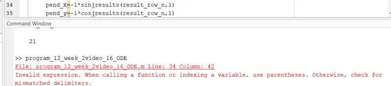
Error 2:Invalid expression. When calling a function or indexing a variable, use parentheses. Otherwise, check for
mismatched delimiters.

Cause:The command called at this line is an invalid expression. MATHLAB can recognize the function, but the syntaxe is not correct. on this line, 2 parentheses are opened, but only 1 was closed.

pend_X=-1*sin(results(result_row_n,1))

Corrective: After looking at the code, I added the missing parenthese at the end.

Part 2 :Upload an animation on You tube and provide the You tube link for an animation in your report.

As requested in the instructions, please follow this link to youtube to see the final video animation.

You tube link:

https://youtu.be/QMGD87C9AGs