Project 1 - Parsing NASA thermodynamic data
Challenge:
Write a function that extracts the 14 co-efficients and calculates the enthalpy, entropy and specific heats for all the species in the data file. You will be reading this file NASA thermodynamic data
The main code:
%This program will extract data from the source file THERMO.dat using
%MATLAB. It will after calculate and analyse thermodynamic features and
%plot graphics, that will saved in a folder.
%Written by Dave Levesque following the video 24, 25 and 26 teaching

%program initalization
clear all % clear all variable from previous programs or previous executions
close all % close all windows, graphics and tables previously generated by mathlab
clc % Clear command window

%Preparing the data

%Coeficients
R=8.31446261815324;  %universal gas constant

%Molecular weight importing

Atomic_name=["H" "C" "O" "N" "AR"];
Atomic_weigth_array= [1.008 12.011 15.999 14.007 39.948];

Element_number = 1;
Element_Data=cell(4,1);

%Element #1

Element=1;
line_number=5;
row=1;
Weight = 0;


%Reading the data file----------------------------------------------------


%Linking the variable 'fthermodata' to the data file
fthermodata=fopen('THERMO.dat','r');

%Reading the line #1
fgetl(fthermodata);

%Reading the line #2
line2=fgetl(fthermodata);
GlobalTempstring=strsplit(line2,' ');

%Processing the data string from line 2
GlobalTemp1=str2num(GlobalTempstring{2});
GlobalTemp2=str2num(GlobalTempstring{3});
GlobalTemp3=str2num(GlobalTempstring{4});

%Reading the 3 comment lines
for i=1:3;
   fgetl(fthermodata);
end


%MAIN  LOOP  ------------------------------------------------------

for k = 1:100;  % Execute 100 times
%Reading the first line of the first element

%Reading the elements (spieces) data, calculating and ploting

species=fgetl(fthermodata);
M=strsplit(species,' ');
name_species=M{1};
Component_Atomic= name_species

%Endind the main loop - if no more Elements found
%----------------------------------
if Component_Atomic == "END";
    break
end
%----------------------------------
%Processing local temp
lowtemp=M{end -3};
midtemp=M{end -2};
hightemp=M{end -1};
lowtemp=str2num(lowtemp);
midtemp=str2num(midtemp);
hightemp=str2num(hightemp);

%getting the coeficients - line by line

%coeficient line 1/3

line2=fgetl(fthermodata);
p1=findstr(line2,'E');
%Coeficient #1
a1=line2(1:p1(1)+3);
a1=str2num(a1);
%Coeficient #2
a2=line2(p1(1)+4:p1(2)+3);
a2=str2num(a2);
%Coeficient #3
a3=line2(p1(2)+4:p1(3)+3);
a3=str2num(a3);
%Coeficient #4
a4=line2(p1(3)+4:p1(4)+3);
a4=str2num(a4);
%Coeficient #5
a5=line2(p1(4)+4:p1(5)+3);
a5=str2num(a5);
%next 5 coeficients on next line
%coeficient line 2/3
line3=fgetl(fthermodata);
p1=findstr(line3,'E');
%Coeficient #6
a6=line3(1:p1(1)+3);
a6=str2num(a6);
%Coeficient #7
a7=line3(p1(1)+4:p1(2)+3);
a7=str2num(a7);
%Coeficient #8
a8=line2(p1(2)+4:p1(3)+3);
a8=str2num(a8);
%Coeficient #9
a9=line2(p1(3)+4:p1(4)+3);
a9=str2num(a9);
%Coeficient #10
a10=line2(p1(4)+4:p1(5)+3);
a10=str2num(a10);
%next 5 coeficients on next line
%coeficient line 3/3
line4=fgetl(fthermodata);
p1=findstr(line4,'E');
%Coeficient #11
a11=line3(1:p1(1)+3);
a11=str2num(a11);
%Coeficient #12
a12=line3(p1(1)+4:p1(2)+3);
a12=str2num(a12);
%Coeficient #13
a13=line3(p1(2)+4:p1(3)+3);
a13=str2num(a13);
%Coeficient #14
a14=line3(p1(3)+4:p1(4)+3);
a14=str2num(a14);

% Enthalpy, Emtropy and Specific heat calculation
%function[H_high]=F_Enthalpy_HIGH_T(R,a1,a2,a3,a4,a5,a6,T_high)
T= linspace(lowtemp,hightemp, 100);
if T >=midtemp;
%Enthalpy
H = a1 + ((a2 .* (T)./2))+((a3.*(T.^2))/3)+((a4.*(Th.^3)./4))+(a5.*((T.^4)./5))+(a6./T).*R.*T;
%Entropy
S =(((a1 .*log(T_high)) + (a2 .* T_high) + (a3 .* T_high.^2 ./2) + (a4 .* T_high.^3 ./3) + ((a5 .* T_high.^4 ./4) + a7) ))*R;
%Specific Heat
Cp =(a1 + a2 * T_high + a3 *T_high.^2 + a4 *T_high.^3 + a5 *T_high.^4)*R;

else
%Enthalpy
H = a8 + ((a9 .* (T)./2))+((a10.*(T.^2))/3)+((a11.*(T.^3)./4))+(a12.*((T.^4)/5))+(a13./T)*R.*T ;
%Entropy
S =(((a8 .*log(T)) + (a9 .* T) + (a10 .* T.^2 ./2) + (a11 .* T.^3 ./3) + ((a12 .* T.^4 ./4) + a14) ))*R;
%Specific Heat
Cp=(a8 + a9 * T + a10 *T.^2 + a11 *T.^3 + a12 *T.^4)*R;
end

%Molecular weight Caculation

%Getting the atoms name and qty of each for this element

%Loop comparing the strings to process atom names and qties
 for i = 1:length(Component_Atomic);

    for j = 1:length(Atomic_name);
        if  strcmp(Component_Atomic(i), Atomic_name(j));
            Weight = Weight + Atomic_weigth_array(j);
            pos= j;
        end
    end

number=str2num(Component_Atomic(i));

if number > 1;
     Weight = Weight + (Atomic_weigth_array(pos)*(number-1));
end

 end
if Weight > 0
disp("Specy Atomic Weight"  )
Weight
end

%Element = next element - incrementing/resetting variables for the next execution

Weight = 0;

%---------------------------------------------------------------
%Plotting the graphics and saving in folders

%Creating a folder and setting directory
cd('C:\Users\Owner\Desktop\MathLab\NASA_species_results' )
mkdir( Component_Atomic )
cd(Component_Atomic)

%Plot Enthalpy H vs Temperature
figure(1)
plot(H,T)
xlabel('Temperature in K')
ylabel( 'Enthalpy in KJ/mol')
title(sprintf('%s','Specie:',name_species,'-Enthalpy vs Temperature'))
saveas(figure(1),'enthalpy.png')

%Plot Entropy S vs Temperature
figure(2)
plot(S,T)
xlabel('Temperature in K')
ylabel('Entropy in KJ/mol-K')
title(sprintf('%s','Specie:',name_species,'-Entropy vs Temperature'))
saveas(figure(2),'entropy.jpg')

%Plot Specific Heat CP vs Temperature
figure(3)
plot(S,T)
xlabel('Temperature in K')
ylabel( 'Specific Heat')
title(sprintf('%s','Specie:',name_species,'-Specific Heat vs Temperature'))
saveas(figure(3),'specific_heat.jpg')

%change working directory
cd('C:\Users\Owner\Desktop\MathLab')


end %end of MAIN LOOP processing all elements


fclose(fthermodata);
%End of program.
Program initialization:
In order to start on a clean slate, the first funtions of my code are the followings, clear all, close all and clc.
clear all : clear all variable from previous programs or previous executions
close all : close all windows, graphics and tables previously generated by matlab
clc : clear command window
Preparing the data:
We are here entering usefull coefients and constants that will be needed in the program.
%Coeficients
R=8.31446261815324; %universal gas constant
These next arrays will be used later for the atomic weigth calculation. We have an array of data in the variables.
Atomic_name=["H" "C" "O" "N" "AR"];
Atomic_weigth_array= [1.008 12.011 15.999 14.007 39.948];
The next step is to open the our source data file and link to a variable that can be called out later. The file supplied to us by NASA is 'THERMO.dat'. The file has been transfered over in the working directoy from where MATLAB is executing this program. Please note that the file name is case sensitive. When using the command 'fopen', the file name argument has to take this in account. The second argument used for the command file open, is 'r', that stands for reading. So we are opening the file with reading permission.
%Linking the variable 'fthermodata' to the data file
fthermodata=fopen('THERMO.dat','r');
The first line of the data file can now be read. This is done using the command 'fgetl', that stands for file get line. The very first line of the data file is read. Since that first line is the title, there is no usefull information to process, we are then calling that same command, that will now read the next line, and store the values in the variable 'line2'. What we got from reading this line 2, is a string with different values in it in one block. In order to separate that information, we are using the comand 'strsplit'. The arguments are the source string, 'line2' and the delimiter we want to use to seperate the string, space in this case. So the string will be split everytime it sees a space in the string. With the string seperated in in different element, in the variable of our choice, we will convert these smaller strings into numeric values, so the program see it as numbers, instead of strings of caracters. The command used is 'str2num'. Note that we have to use the curly brackets on that line of code. We see next a loop that will be used to read the next three lines, that do not have to be processed, just read.
%Reading the line #1
fgetl(fthermodata);
%Reading the line #2
line2=fgetl(fthermodata);
GlobalTempstring=strsplit(line2,' ');
%Processing the data string from line 2
GlobalTemp1=str2num(GlobalTempstring{2});
GlobalTemp2=str2num(GlobalTempstring{3});
GlobalTemp3=str2num(GlobalTempstring{4});
%Reading the 3 comment lines
for i=1:3;
fgetl(fthermodata);
end
Leading into the main section of the program, the main loop is taking place. For every execution of this loop, the speicie data will be read, the values of S, H, and CP will be calculated, the molecular weight will be calculated and the curves will be plotted and saved. Then the loop will execute again with the following speicie, until the end. The same principle as in the first section of the program is being used here, using the commands 'fgetl', 'strsplit'. In the case where are done reading the the species, we will have 'END' for specie name. Using a 'if' statement, we are testing that condition at every execution. When the condition is true, then the main loop will be stopped, using the 'break' function.
%MAIN LOOP ------------------------------------------------------
for k = 1:100; % Execute 100 times
%Reading the first line of the first element
%Reading the elements (spieces) data, calculating and ploting
species=fgetl(fthermodata);
M=strsplit(species,' ');
name_species=M{1};
Component_Atomic= name_species
%Endind the main loop - if no more Elements found
%----------------------------------
if Component_Atomic == "END";
break
end
%----------------------------------
The local temperature were read at the same time as the specie's name, because it is on the same line on the data file. We see that the temperatures are always the last 4 numbers on the line, from the end. Because the number of data on this string is variable from one specie to another, we could not simply use the the position of the temperature from the begining of the line. We noticed that counting the postion from the end was a consistent way to indicate the postion of the low, mid and high temperature.
%Processing local temp
lowtemp=M{end -3};
midtemp=M{end -2};
hightemp=M{end -1};
lowtemp=str2num(lowtemp);
midtemp=str2num(midtemp);
hightemp=str2num(hightemp);
The fourteen coeficient nescerary for the next step are now being read, stored and converted. The coeficients are found on three different lines in the data file, having 5 on the first two lines and the remaining the on third line. After reading the line, a custom string split is done. We are using the 'E' as the delimiter. The position of each letter 'E' is found and stored in a variable. The them we are using the positions of 'E' stored in the array of variable 'p1' to determine where our usefull pieces of the strings are. We know that the coeficient begins four caracters after the previous one, and three caracters after the current one. The delimitation can be done and the results store in the variables, 'a1 to a8'. The command 'str2num' is used the convert the data contained in each of the variables so it can be used for calculations later. The have to proceed line by line, reading it, splitting the data, and then reading the next line.
%getting the coeficients - line by line
%coeficient line 1/3
line2=fgetl(fthermodata);
p1=findstr(line2,'E');
%Coeficient #1
a1=line2(1:p1(1)+3);
a1=str2num(a1);
%Coeficient #2
a2=line2(p1(1)+4:p1(2)+3);
a2=str2num(a2);
%Coeficient #3
a3=line2(p1(2)+4:p1(3)+3);
a3=str2num(a3);
%Coeficient #4
a4=line2(p1(3)+4:p1(4)+3);
a4=str2num(a4);
%Coeficient #5
a5=line2(p1(4)+4:p1(5)+3);
a5=str2num(a5);
%next 5 coeficients on next line
%coeficient line 2/3
line3=fgetl(fthermodata);
p1=findstr(line3,'E');
%Coeficient #6
a6=line3(1:p1(1)+3);
a6=str2num(a6);
%Coeficient #7
a7=line3(p1(1)+4:p1(2)+3);
a7=str2num(a7);
%Coeficient #8
a8=line2(p1(2)+4:p1(3)+3);
a8=str2num(a8);
%Coeficient #9
a9=line2(p1(3)+4:p1(4)+3);
a9=str2num(a9);
%Coeficient #10
a10=line2(p1(4)+4:p1(5)+3);
a10=str2num(a10);
%next 5 coeficients on next line
%coeficient line 3/3
line4=fgetl(fthermodata);
p1=findstr(line4,'E');
%Coeficient #11
a11=line3(1:p1(1)+3);
a11=str2num(a11);
%Coeficient #12
a12=line3(p1(1)+4:p1(2)+3);
a12=str2num(a12);
%Coeficient #13
a13=line3(p1(2)+4:p1(3)+3);
a13=str2num(a13);
%Coeficient #14
a14=line3(p1(3)+4:p1(4)+3);
a14=str2num(a14);
We have all the data available now to being the calculation on the Enthalpy and specific heat. There is a particularity with these formulas. It is using different coeficients depending on the temperature being input. If the temperature is between the low and mid range, we have to use the low temperature coeficients, 'a1 to a7'. Else, if the temperature is above the mid to the high limit, we have to calculate our results using the coeficients a8 to a14'.
% Enthalpy, Emtropy and Specific heat calculation
%function[H_high]=F_Enthalpy_HIGH_T(R,a1,a2,a3,a4,a5,a6,T_high)
T= linspace(lowtemp,hightemp, 100);
if T >=midtemp;
%Enthalpy
H = a1 + ((a2 .* (T)./2))+((a3.*(T.^2))/3)+((a4.*(Th.^3)./4))+(a5.*((T.^4)./5))+(a6./T).*R.*T;
%Entropy
S =(((a1 .*log(T_high)) + (a2 .* T_high) + (a3 .* T_high.^2 ./2) + (a4 .* T_high.^3 ./3) + ((a5 .* T_high.^4 ./4) + a7) ))*R;
%Specific Heat
Cp =(a1 + a2 * T_high + a3 *T_high.^2 + a4 *T_high.^3 + a5 *T_high.^4)*R;
else
%Enthalpy
H = a8 + ((a9 .* (T)./2))+((a10.*(T.^2))/3)+((a11.*(T.^3)./4))+(a12.*((T.^4)/5))+(a13./T)*R.*T ;
%Entropy
S =(((a8 .*log(T)) + (a9 .* T) + (a10 .* T.^2 ./2) + (a11 .* T.^3 ./3) + ((a12 .* T.^4 ./4) + a14) ))*R;
%Specific Heat
Cp=(a8 + a9 * T + a10 *T.^2 + a11 *T.^3 + a12 *T.^4)*R;
end
To calculate the molecular weight, it is needed to break down the specie name into its elements, and the number of each element where there is more than 1 of the same element. This done by comparing each atomic symbol with a pre determined list, contained in a variable with established at the beginning of the program. This is done for the first atomic letter, then it is matched with the one in our reference list. We know the postion of this value in the array of the variable, that we can after match with the other array, containing the respective weight for this atom. The variable weight is updated with that found weight being added. Then, the program goes to another loop to compare if the caracter being evaluated is a valid number greater than 1. If yes, that means we have more that one of the same atom. That number of atom is multiplied by the weight and then added on to the 'weight' variable. The last five lines are used to display the atomic weight and name of the species, unless there is no valid weight found.
%Molecular weight Caculation
%Getting the atoms name and qty of each for this element
%Loop comparing the strings to process atom names and qties
for i = 1:length(Component_Atomic);
for j = 1:length(Atomic_name);
if strcmp(Component_Atomic(i), Atomic_name(j));
Weight = Weight + Atomic_weigth_array(j);
pos= j;
end
end
number=str2num(Component_Atomic(i));
if number > 1;
Weight = Weight + (Atomic_weigth_array(pos)*(number-1));
end
end
if Weight > 0
disp("Specy Atomic Weight" )
Weight
end
Generating the graphics, files and folders.
Before generatic the plots and saving the files, the program is directing MATLAB in the folder where we want the folders to be created in. I created the folder 'NASA_species_results' for the purpose of storing the species folders in an organized way. The command 'cd' is used here. It stands for change directory. Next we are introducing the next command, 'mkdir'. It stands for Make Directory, and the argument provided is the here the name of the new directory to be created. The variable 'Component_Atomic', which stores the name of the specie will be used for naming the folder for each specie. Once the new directory, folder, is created, we are using again 'cd' to move the active working directory of MATLAB in this new folder.
%Creating a folder and setting directory
cd('C:\Users\Owner\Desktop\MathLab\NASA_species_results' )
mkdir( Component_Atomic )
cd(Component_Atomic)
Everything is ready to proceed with each of the three plots for the values of H,S and CP versus temperature. The command 'saveas' will be used after each plot, using the arguments 'figure(x)' and file name.
%Plot Enthalpy H vs Temperature
figure(1)
plot(H,T)
xlabel('Temperature in K')
ylabel( 'Enthalpy in KJ/mol')
title(sprintf('%s','Specie:',name_species,'-Enthalpy vs Temperature'))
saveas(figure(1),'enthalpy.png')
%Plot Entropy S vs Temperature
figure(2)
plot(S,T)
xlabel('Temperature in K')
ylabel('Entropy in KJ/mol-K')
title(sprintf('%s','Specie:',name_species,'-Entropy vs Temperature'))
saveas(figure(2),'entropy.jpg')
%Plot Specific Heat CP vs Temperature
figure(3)
plot(S,T)
xlabel('Temperature in K')
ylabel( 'Specific Heat')
title(sprintf('%s','Specie:',name_species,'-Specific Heat vs Temperature'))
saveas(figure(3),'specific_heat.jpg')
After the execution of the lines aboves, we need to change back the working directory of MATLAB in preparation of the next 'Main Loop' execution.
%change working directory
cd('C:\Users\Owner\Desktop\MathLab')
And the main loop is now ending here, it will execute 100 times or until the specie 'END' is detected.
end %end of MAIN LOOP processing all elements
One last thing before ending this program, is the need to close the source data file. It is done using the command 'flclose', file close.
fclose(fthermodata);
%End of program.
Results-generated by the program
Calculate the molecular weight of each species and display it in the command window. A few example shown here.
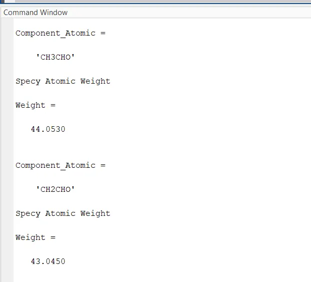
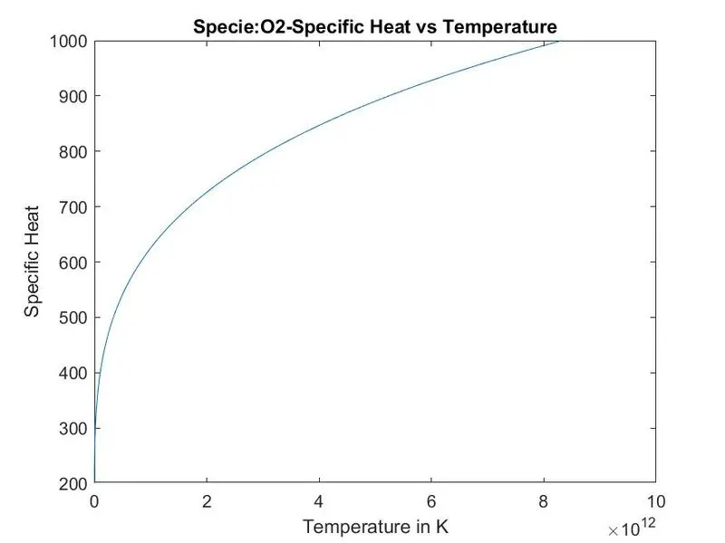
Plots for o2, N2 and Co2 species
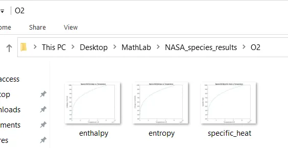
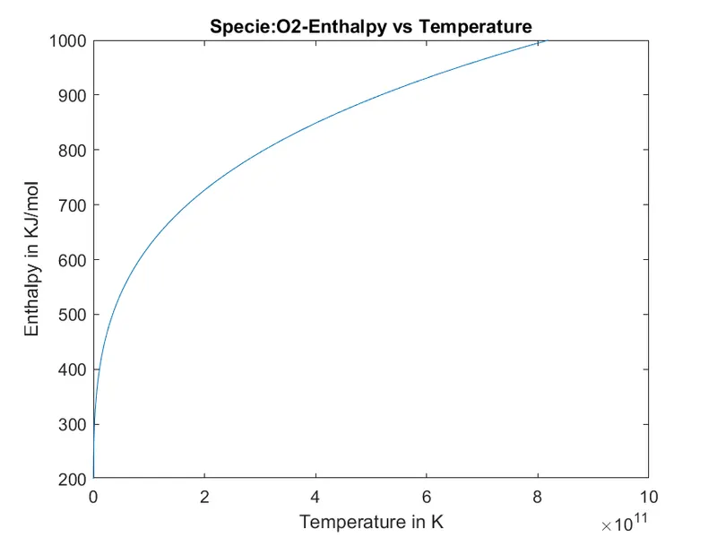
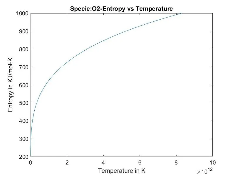
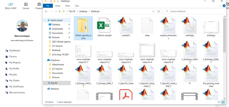
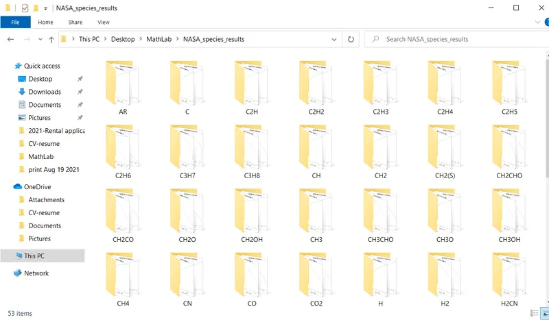
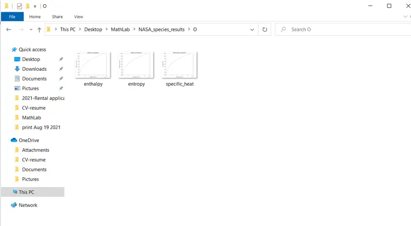
Folders and saved plots of each specie
Conclusion- lessons learned.
My first version of the program was very long and complex to achieve a similar results. With the help of my teacher, I ended up with this final version, that is much more robust, simple, shorter and efficent. I learned a lot by trying to find out a good solution on my own and I will retain that extra knowledge and the extra time was not wasted.
Errors faced while programing:
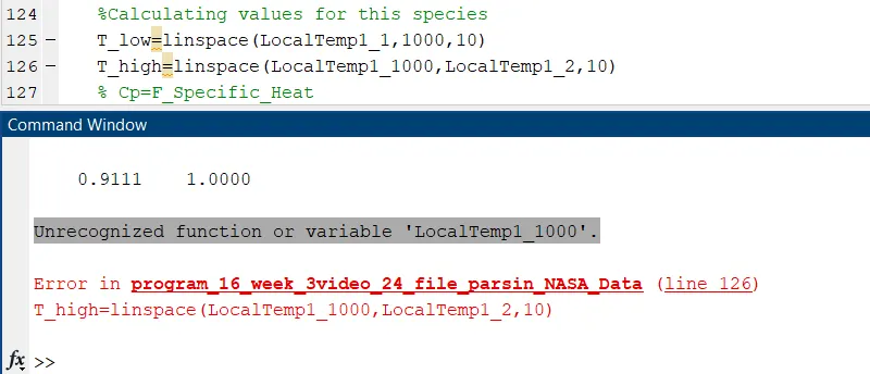
Error 1:Unrecognized function or variable 'LocalTemp1_1000'.
Cause: MATLAB is unable to process that line of operations. It could be because of a missing ',' or invalid delemiter. The function 'linspace' is requiring the following syntaxe: y = linspace(x1,x2,n).
Corrective: Once the function spelled and typed in correctly, it was recongnized by MATLAB and the error was gone.
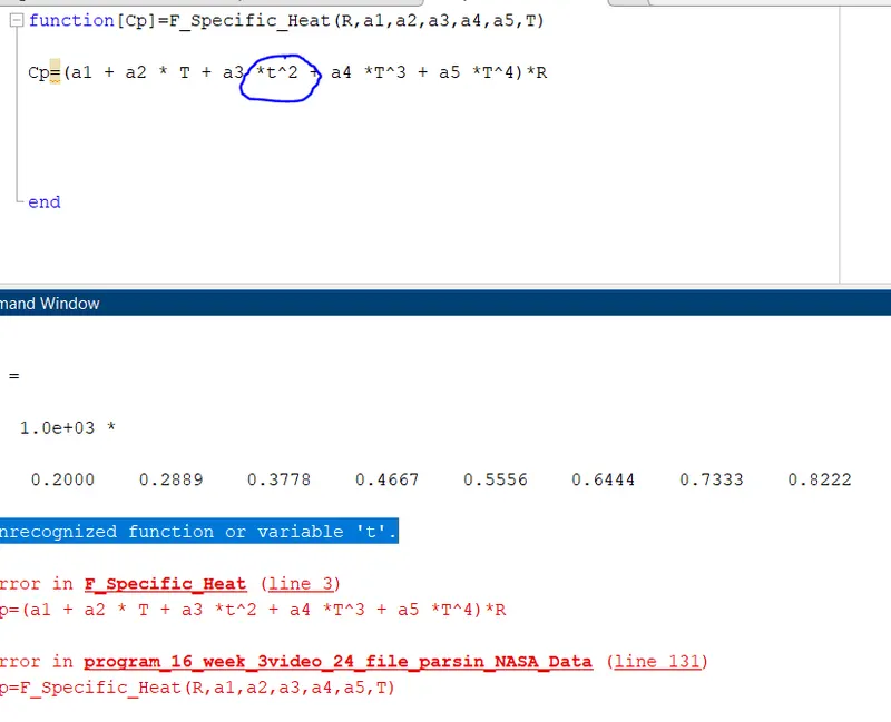
Error 2: Unrecognized function or variable 't'.
Cause: MATLAB is unable to process that line of operations because the variable 't' is not recongnized. The variable ' T ' has been declared, but a typo mistake slipped in, using a small caracter ' t ' instead of the capital letter. MATLAB variable names are case sensitives.
Corrective: Once the variable name spelled and typed in correctly, it was recongnized by MATLAB and the error was gone.
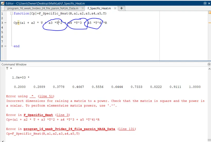
Error 3:Error using ^ (line 51) Incorrect dimensions for raising a matrix to a power. This error is caused by a missing '.' before the power symbol '^'.
Corrective: MATLAB is also stating the error message a good possbile resolution for this error: "To perform elementwise matrix powers, use '.^'. " After adding the ' . ' before the exposant the problem has been solved.
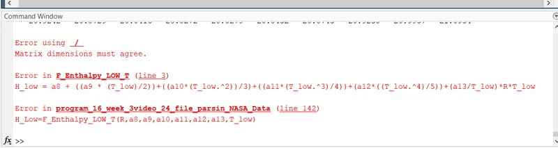
Error 4: 'Error using /' , 'Matrix dimensions must agree.'
Cause: The reason was that I used matrix division instead of element-by-element division. Adding the ' . ' specify to MATLAB we want to do an element by element multiplication or division rathen then by matrix. This why the error message says the matrix dimension don't match.
Corrective: After adding the dot where required, it fixed the error.
References