Project 2 - Rankine cycle Simulator
Challenge:
- Create a Rankine Cycle Simulator using OCTAVE/MATLAB.
- Your code should calculate the state points of the Rankine Cycle (any type of your choice) based on user inputs.
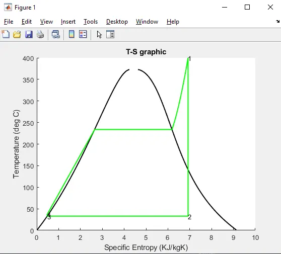
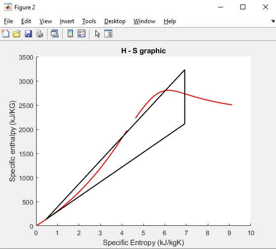
- Then, plot the corresponding T-s and h-s plots for the given set of inputs. Title and axes labels are a must, while legends could be used if necessary.
- The presentation of your code will be taken into consideration while grading. Labelling sections of your code using comments is appreciated.
- Attach a report explaining the working of a rankine cycle simulator and also the research done by you.
Introduction to the Rankine Cycle
"The Rankine cycle is named after William John Macquorn Rankine, a Scottish polymath professor at Glasgow University."
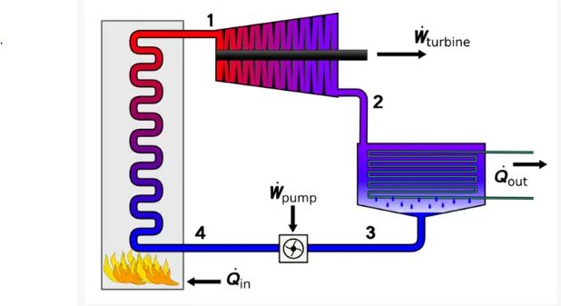
It is the ideal thermodynamic cycle describing the process of producing mechanical energy from a fluid that is going up and down in temperature. In our case, we will consider a system where the heat source is a boiler, heating the fluid, water, turning it into stream. Then the steam is fed through a turbine producing mechanical work. The steam exhausting from the turbin then goes through a condenser. Heat will be sunk our in the atmosphere and the steam will turn back into water. In order to put the water back in the boiler, it needs to pumped to at least the same pressure as inside the boiler. This pump is using some mechanical energy to accomplish this task.
1-The code
%This program will experiment with the Ideal Rankine Cycle using MATLAB
%The add on module/library X Steam is being used for the specifics
%calculations
%Written by Dave Levesque Oct 2021

%program initalization
clear all % clear all variable from previous programs or previous executions
close all % close all windows, graphics and tables previously generated by mathlab
clc % Clear command window

%Preparing the data - Display user text in collecting inputs

disp('        Rankine Cycle Simulator  ')
disp('        Ideal Thermodynamic Cycle  ')
disp('           ')

% Inputs from user - Prompt user the enter the starting values
disp('      Starting data input      ')
disp('           ')
% P1 - Boiler outlet - Turbine Inlet
p1 = input('Enter pressure at boiler Outlet-Turbine Inlet, in bar: ');
%Temperature boiler Outlet - Turbine Inlet
T1 = input('Enter Temperature boiler Outlet - Turbine Inlet, in celcius: ');
%Pressure at the outlet of the turbine - in bar
p2 = input('Enter Pressure at the outlet of the turbine, in bar: ');
disp('           ')

% Calculating the values at P1 - Boiler Outler - Turbine inlet

%Specific entropy
s1 = XSteam ( 's_pT', p1, T1 );
%enthalpy p1 from pressure and temperature
h1 = XSteam ( 'h_pT', p1, T1 );
%Temperature of saturation
tsat1 = XSteam ( 'tsat_p', p1);
%Specific entropy - sL_p  Saturated liquid entropy
sf1 = XSteam ( 'sL_p',p1 );
%Specific entropy -sV_p	Saturated vapour entropy
sg1 = XSteam ( 'sV_p',p1 );

%Testing if the steam is saturated or super heated (dry)
if T1 > tsat1
 %enthalpy p1 from pressure and temperature
 h1 = XSteam ( 'h_pT', p1, T1 );
 %Specific entropy
 s1 = XSteam ( 's_pT', p1, T1 );

elseif T 1== tsat1
 h1 = XSteam ('hL_p', p1)   ;
 s1 = XSteam ('sL_p', p1)  ;

else
    disp('temperature too low under the saturation point')
end


% P2 - Turbine outlet
% Calculating the values at P2 - Turbine Outlet - Condenser inlet
s2=s1;
%Specific entropy - sL_p  Saturated liquid entropy
sf2 = XSteam ( 'sL_p',p2 );
%Specific entropy -sV_p	Saturated vapour entropy
sg2 = XSteam ( 'sV_p',p2 );
%Enthalpy - Saturated liquid enthalpy
hf2 = XSteam ( 'hL_p',p2 );
%Enthalpy -Saturated vapour enthalpy
hg2 = XSteam ( 'hV_p', p2 );
%Temperature T2 Saturated steam
T2 = XSteam ( 'Tsat_p', p2 );
%Vapour fraction - x -Dryness
x2 = ((s2-sf2)/(sg2-sf2));
%Enthalpy - factoring in the dryness/wetness ratio
h2 =  hf2+(x2*(hg2-hf2));


%P3 - Condenser outlet - Pump Inlet saturated liquid
% Pressure
p3 = p2;
%Specific entropy - sL_p  Saturated liquid entropy
s3 = XSteam ( 'sL_p', p3 );
%Enthalpy -Saturated vapour enthalpy
h3 = XSteam ( 'h_ps' , p3, s3);
% Temperature
T3 = T2;


%P4 - Pump outlet - Boilet inlet
%pressure
p4 = p1;
%Specific entropy - sL_p  Saturated liquid entropy
s4 = s3;
%Entalpy as a function of pressure and entropy
h4 = XSteam( 'h_ps', p4,s4 );

% Cp-Specific isobaric heat capacity
Cp4 = XSteam ('Cp_ps', p4,s4);
% Cv	Specific isochoric heat capacity
Cv4 = XSteam ('CV_ps',p4,s4);

%Temperature Calulation
gamma = Cp4/Cv4;
T4 = T3*(p4/p3)^((gamma-1)/gamma);


% System overall Calculation _______________________________________

% Work done by the pump
%vL_p	Saturated liquid volume
v3 = XSteam('vL_p',p3);
% work pump
wp = v3*(p4-p3)*100;
% Work from the Turbine
wt=h1-h2;

% Heat Input burner - boiler source of heat
qin = h1 - h4;

%Heat output rejected by the condensor
qout = h2-h3;

%Net Work
wnet= wt - wp;

%Thermodynamic efficency
td_eff = (wnet/qin)*100;

%Plotting the diagrams ____________________________________________
% T - S
figure(1)
hold on
%plotting saturation lines
temp = linspace(1, 373, 500);

hl=zeros(1,100);
hv=zeros(1,100);
sl=zeros(1,100);
sv=zeros(1,100);

for i = 1 : length(temp)
    hl(i) = XSteam('hL_T',temp(i));
    hv(i) = XSteam('hV_T',temp(i));
    sl(i) = XSteam('sL_T',temp(i));
    sv(i) = XSteam('sV_T',temp(i));
end

plot(sl,temp, 'K','linewidth',1.5)
plot(sv,temp, 'K','linewidth',1.5)
xlabel('Specific Entropy (KJ/kgK)')
ylabel('Temperature (deg C)')
title('T-S graphic')
plot([s1 s2 s3 s4 sf1 sg1],[T1 T2 T3 T4 tsat1 tsat1], 'color', 'g', 'linewidth', 1.5)
text(s1,T1, '1')
text(s2,T2, '2')
text(s3,T3, '3')
text(s4,T4, '4')
t = linspace(tsat1, T1, 1000);
 for j = 1 : length(t)
 sp(j) = XSteam('S_pT', p1, t(j));
 end
 plot(sp,t, 'color', 'g', 'linewidth',1.5)


% H - S

figure(2)
hold on
title('H - S graphic')
xlabel('Specific Entropy (kJ/kgK)')
ylabel('Specific enthalpy (kJ/KG)')
plot(sl,hl, 'r', 'linewidth',1.5)
plot(sv,hv, 'r', 'linewidth',1.5)
plot([s1 s2 s3 s4 s1],[h1 h2 h3 h4 h1], 'color', 'black', 'linewidth',1.5)


%Priting the output results ____________________________________________

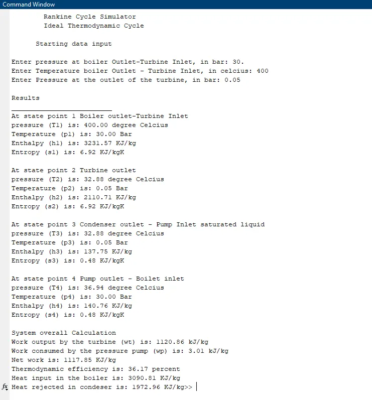
disp(     'Results'      )
disp(   '_________________________'      )

%State 1
disp('At state point 1 Boiler outlet-Turbine Inlet')
fprintf('pressure (T1) is: %.2f degree Celcius', T1)
fprintf('\nTemperature (p1) is: %.2f Bar', p1)
fprintf('\nEnthalpy (h1) is: %.2f KJ/kg', h1)
fprintf('\nEntropy (s1) is: %.2f KJ/kgK\r\n', s1)

%State 2
disp('At state point 2 Turbine outlet')
fprintf('pressure (T2) is: %.2f degree Celcius', T2)
fprintf('\nTemperature (p2) is: %.2f Bar', p2)
fprintf('\nEnthalpy (h2) is: %.2f KJ/kg', h2)
fprintf('\nEntropy (s2) is: %.2f KJ/kgK\r\n', s2)

%State 3
disp('At state point 3 Condenser outlet - Pump Inlet saturated liquid')
fprintf('pressure (T3) is: %.2f degree Celcius', T3)
fprintf('\nTemperature (p3) is: %.2f Bar', p3)
fprintf('\nEnthalpy (h3) is: %.2f KJ/kg', h3)
fprintf('\nEntropy (s3) is: %.2f KJ/kgK\r\n', s3)

%State 4
disp('At state point 4 Pump outlet - Boilet inlet')
fprintf('pressure (T4) is: %.2f degree Celcius', T4)
fprintf('\nTemperature (p4) is: %.2f Bar', p4)
fprintf('\nEnthalpy (h4) is: %.2f KJ/kg', h4)
fprintf('\nEntropy (s4) is: %.2f KJ/kgK\r\n', s4)

%System overall Calculation
disp('System overall Calculation')
fprintf('Work output by the turbine (wt) is: %.2f kJ/kg',wt)
fprintf('\nWork consumed by the pressure pump (wp) is: %.2f kJ/kg',wp)
fprintf('\nNet work is: %.2f KJ/kg', wnet)
fprintf('\nThermodynamic efficiency is: %.2f percent',td_eff)
fprintf('\nHeat input in the boiler is: %.2f KJ/kg', qin)
fprintf('\nHeat rejected in condeser is: %.2f KJ/kg',qout)


%The end of the code
2-Code Explained:
Program initialization:
In order to start on a clean slate, the first funtions of my code are the followings, clear all, close all and clc.
clear all : clear all variable from previous programs or previous executions
close all : close all windows, graphics and tables previously generated by matlab
clc : clear command window
Getting the initial datas
To begin the resolution of the problem, the three following parameters are entered by the user, p1, T1 and p2. To to do, we are using the command 'input'. The user is seeing a prompt text, asking for the data needed from us, and the proper unit is specified. On this challenge, the command window is used as a user interface, to enter the starting data, and to display the results later on.
%Preparing the data - Display user text in collecting inputs
disp(' Rankine Cycle Simulator ')
disp(' Ideal Thermodynamic Cycle ')
disp(' ')
% Inputs from user - Prompt user the enter the starting values
disp(' Starting data input ')
disp(' ')
% P1 - Boiler outlet - Turbine Inlet
p1 = input('Enter pressure at boiler Outlet-Turbine Inlet, in bar: ');
%Temperature boiler Outlet - Turbine Inlet
T1 = input('Enter Temperature boiler Outlet - Turbine Inlet, in celcius: ');
%Pressure at the outlet of the turbine - in bar
p2 = input('Enter Pressure at the outlet of the turbine, in bar: ');
disp(' ')
3-Calculating the state point
To calculate the parameters of the Rankine cycle at state points, were using the library X Steam. It has all the formula in shape of functions built in for us to use. All there is to do, is to call the needed function with its required arguments. The process is repeated in similarly for the state point 2,3 and 4.
% Calculating the values at P1 - Boiler Outler - Turbine inlet
%Specific entropy
s1 = XSteam ( 's_pT', p1, T1 );
%enthalpy p1 from pressure and temperature
h1 = XSteam ( 'h_pT', p1, T1 );
%Temperature of saturation
tsat1 = XSteam ( 'tsat_p', p1);
%Specific entropy - sL_p Saturated liquid entropy
sf1 = XSteam ( 'sL_p',p1 );
%Specific entropy -sV_p Saturated vapour entropy
sg1 = XSteam ( 'sV_p',p1 );
There is a specific step here at this stage of State point 1. The Rankine cycle simulation here is based on a ideal configuration. That implies that the steam coming out of the boiler is at a Super Heated state. This kind of steam is also called Dry Steam. In the situation where the user wants to run this simulation with numbers not creating this conditions, the ideal Rankine cycle cannot be done the same way. This is why I added the 'if' statement to test that condition. If the user is entering a boiler outlet temperature that would too low to obtain saturated steam, a message will be displayed to explain this condition.
%Testing if the steam is saturated or super heated (dry)
if T1 > tsat1
%enthalpy p1 from pressure and temperature
h1 = XSteam ( 'h_pT', p1, T1 );
%Specific entropy
s1 = XSteam ( 's_pT', p1, T1 );
elseif T 1== tsat1
h1 = XSteam ('hL_p', p1) ;
s1 = XSteam ('sL_p', p1) ;
else
disp('temperature too low under the saturation point')
end
The parameters for the other State Points are calculated to further use and display.
4-system overall calculations
Here is calculated the parameters for the whole system, based on the datas from the different state points. Once again, the library X Steam is really great at resolving our parameters using its functions.
% Work done by the pump
%vL_p Saturated liquid volume
v3 = XSteam('vL_p',p3);
% work pump
wp = v3*(p4-p3)*100;
% Work from the Turbine
wt=h1-h2;
% Heat Input burner - boiler source of heat
qin = h1 - h4;
%Heat output rejected by the condensor
qout = h2-h3;
%Net Work
wnet= wt - wp;
%Thermodynamic efficency
td_eff = (wnet/qin)*100;
5-Plotting the diagrams
The code below is used to generate the graphics, for T-S and H-S. Note here that we are using the command ' zeros ' for the first time. It will create an array with all values filled with 0. That allows to create a defined sized varialbe array, when the values are not yet know.
% T - S
figure(1)
hold on
%plotting saturation lines
temp = linspace(1, 373, 500);
hl=zeros(1,100);
hv=zeros(1,100);
sl=zeros(1,100);
sv=zeros(1,100);
for i = 1 : length(temp)
hl(i) = XSteam('hL_T',temp(i));
hv(i) = XSteam('hV_T',temp(i));
sl(i) = XSteam('sL_T',temp(i));
sv(i) = XSteam('sV_T',temp(i));
end
plot(sl,temp, 'K','linewidth',1.5)
plot(sv,temp, 'K','linewidth',1.5)
xlabel('Specific Entropy (KJ/kgK)')
ylabel('Temperature (deg C)')
title('T-S graphic')
plot([s1 s2 s3 s4 sf1 sg1],[T1 T2 T3 T4 tsat1 tsat1], 'color', 'g', 'linewidth', 1.5)
text(s1,T1, '1')
text(s2,T2, '2')
text(s3,T3, '3')
text(s4,T4, '4')
t = linspace(tsat1, T1, 1000);
for j = 1 : length(t)
sp(j) = XSteam('S_pT', p1, t(j));
end
plot(sp,t, 'color', 'g', 'linewidth',1.5)
% H - S
figure(2)
hold on
title('H - S graphic')
xlabel('Specific Entropy (kJ/kgK)')
ylabel('Specific enthalpy (kJ/KG)')
plot(sl,hl, 'r', 'linewidth',1.5)
plot(sv,hv, 'r', 'linewidth',1.5)
plot([s1 s2 s3 s4 s1],[h1 h2 h3 h4 h1], 'color', 'black', 'linewidth',1.5)
6-Priting the output results
Having all the parameters resolved, now all that is left is to display it the command window. The display command is used to show text to the user.
disp('At state point 1 Boiler outlet-Turbine Inlet')
To display the values from the variables, the function fprintf is used, with the argument '%.2f' This means we want to display the number in a floating point format, with 2 decimals. We also print a string of text in betwneen the quote signs ' ' .
fprintf('Work output by the turbine (wt) is: %.2f kJ/kg',wt)
Errors ecountered
'Unrecognized function or variable 'x2'.
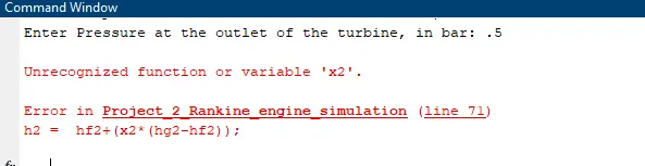
Cause: The variable 'x2' is not defined, or unable to be located by MATLAB. Although, it is defined in the code of the program.
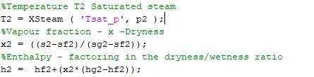
Resolution: I found out that 'x2' was defined AFTER the line of code giving the error. This is why it cannot be found. The code is executed line by line, beginning from the top and going down. Moving the line where 'x2' is defined before resolved the issue.
References:
https://en.wikipedia.org/wiki/Rankine_cycle
https://www.youtube.com/watch?v=biHGK7lbxC0&t=2016s
https://skill-lync.com/student-projects/Rankine-Cycle-10117