Week 4.1 - Genetic Algorithm

AIM : Optimising stalagmite function using MATLAB and to find global maxima.

Objectives of the project :

• To perform a program for calucating population using (genetic algorithm)in MATLAB code.
• Plotting the 3 studies for F maximum vs no of iterations.

INTRODUCTION :

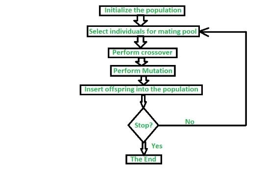
1. Genetic algorithm are part of evalutionary computing,which is rapidly growing area of artifical intelligence.
2. Genetic algorithm (GA)'s are a technique to solve problems which need optimization.
3. GA's are derived from dravin's theory of evaluation.

what is GA ?

Computer models based on genetics which attempt to solve complex problems having many potential solutions by efficiently searching the solution space for optimal or near optimal solutions.

• Incorporate evalution of features

1. survival of fittness
2. crossover
3. mutation

• Iterative process of improvement

syntax for ga :

Syntax
x = ga(fun,nvars)
x = ga(fun,nvars,A,b)
x = ga(fun,nvars,A,b,Aeq,beq)
x = ga(fun,nvars,A,b,Aeq,beq,lb,ub)
x = ga(fun,nvars,A,b,Aeq,beq,lb,ub,nonlcon)
x = ga(fun,nvars,A,b,Aeq,beq,lb,ub,nonlcon,options)
x = ga(fun,nvars,A,b,[],[],lb,ub,nonlcon,IntCon)
x = ga(fun,nvars,A,b,[],[],lb,ub,nonlcon,IntCon,options)
x = ga(problem)
[x,fval] = ga(___)

BODY OF THE CONTENT :

FORMULA :

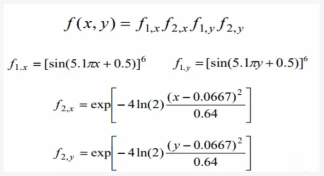
function [f] = stalagmite(input_vector)
x = input_vector(1);
y = input_vector(2);
f1 = (sin(5.1*pi*x + 0.5))^6;
f2 = exp(-4*log(2).*(x- 0.0667)^2/0.64);
f3 = (sin(5.1*pi*y + 0.5))^6;
f4 = exp(-4*log(2).*(y- 0.0667)^2/0.64);
[f] = -(f1.*f2.*f3.*f4);
end

• writing stalagmite function from formula given
• while in the function we use -ve sign ie for that ga only consider only minimum values so -ve sign do reverse the formula and helps us to find global maxima .

MAIN BODY OF THE PROGRAM :

• Defining the function with common commands and giving search commands.
• creating a 1D array to 2D array [X,Y] using meshgrid i,e divides equal parts of x,y values
• surfc command is used to visuialize the plot in 3D view.
• shading interp is used to removeline produced by meshgrid.
• finally,end is used to close the loop.

clear all 
close all
clc
 %search space
 x = linspace(0,0.6,150);
 y = linspace(0,0.6,150);
 n_c=50;
%2D array
 [X,Y] = meshgrid(x,y);

for i=1:length(X)
    for j = 1:length(Y)
        input_vector(1)=X(i,j);
        input_vector(2)=Y(i,j);
        f(i,j) = stalagmite(input_vector);
    end
end
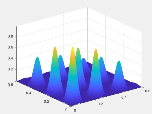
 surfc(X,Y,-f)
 shading interp

RESULT :

STUDY 1 defines the statistical study without boundation

• Here tic and toc is used to calculate the study time taken.
• In evaluating optimum value of the fitness function for each iterations and caluculating using above syntax.

%study 1
 tic
 for i=1:n_c
     [input,fopt(i)] = ga(@stalagmite,2);
     xopt(i)=input(1);
     yopt(i)=input(2);
 end
 study_time1 = toc
 
% %plotting
 figure(1)
 subplot(2,1,1)
 surfc(X,Y,-f)
 hold on
 shading interp
 plot3(xopt,yopt,-fopt,'marker','o','markersize',5,'markerfacecolor','r')
 xlabel('x')
 ylabel('y')
 subplot(2,1,2)
 plot(-fopt)
 xlabel('iterations')
 ylabel('function min')

RESULTS FOR STUDY 1 :

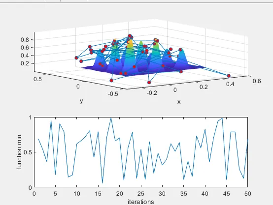
STUDY 2 defines statistical study with boundation

• Here upper and lower boundary limits are given and plotted as same as above study.

 %study2
  tic
  for j=1:n_c
      [input,fopt(j)] = ga(@stalagmite,2,[],[],[],[],[0;0],[1;1]);
      xopt(j)=input(1);
      yopt(j)=input(2);
  end
  study_time2=toc
  
  %plotting
  figure(2)
  subplot(2,1,1)
  hold on
  surfc(X,Y,-f)
  shading interp
  plot3(xopt,yopt,-fopt,'marker','o','markersize',5,'markerfacecolor','r')
  xlabel('x');
  ylabel('y');
  subplot(2,1,2)
  plot(-fopt)
  xlabel('iterations')
  ylabel('function min')

RESULTS FOR STUDY 2 :

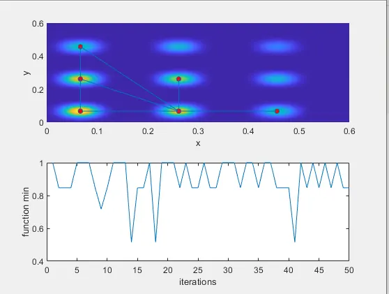
Another 3D view of figure(2):

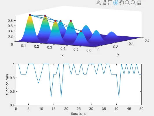
• here the varying in boundary limits is observed clearly after giving the boundary conditions.

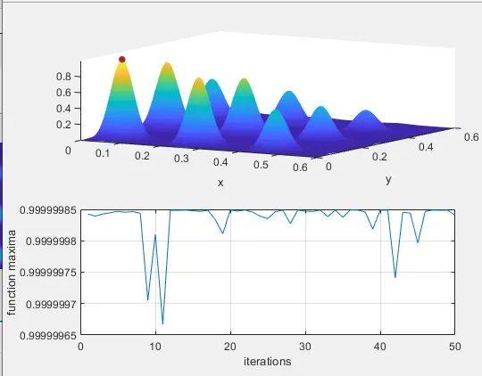
STUDY 3 with increase in size of population.

• Giving the options to ga to caluculate.
• and defining the population size.

 %study3 increasing GA iterations
 options=optimoptions('ga');
 options=optimoptions(options,'populations',300);
 
 tic
 for k=1:n_c
     [input,fopt(k)] = ga(@stalagmite,2,[],[],[],[],[0;0],[1;1],[],[],options);
     xopt(k)=input(1);
     yopt(k)=input(2);
 end
 study_time3=toc
 %plotting
 figure(3)
 subplot(2,1,1)
 hold on
 surfc(X,Y,-f)
 shading interp
 plot3(xopt,yopt,-fopt,'marker','o','markersize',5,'markerfacecolor','r')
 xlabel('x')
 ylabel('y')
 subplot(2,1,2)
 plot(-fopt)
 grid on
 xlabel('iterations')
 ylabel('function maxima')

RESULTS FOR STUDY 3 :

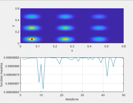
Another 3D view of figure(3) :

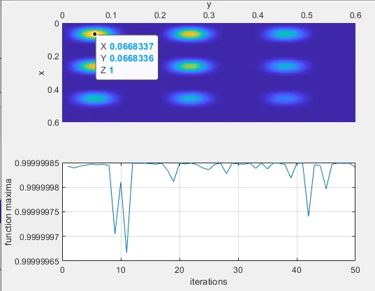
DEFINING X ,Y AND Z VALUES OF GLOBAL MAXIMA :