Week 4.1 - Genetic Algorithm

WHAT IS GENETIC ALGORITHM

It is a algorithm based on the famous Charles Darwin's theory of natural selection. The algorithm reflects the process of natrual selection where the fittest individuals are selected for crossover to produce offspring for the next generation.

It is an intelligent approch of random search provided with data to direct the search into the region of better performance in solution space.

Genetic algorithm is use for optimization purpose along with mathematical function to find the best solution. It is use in the field of Mechanical Engineering to optimize design to the reach desire point of performance for the given conditions. It is widely use in Artificial Inteligence and Machine Learning.

WHAT ARE THE MAIN PHASES OF GENETIC ALGORITHM

1. Initial population.
2. Fittness Function.
3. Selection.
4. Crossover.
5. Mutation.

Brief idea about the above points are given below

• INTIAL POPULATION - It is an array of individuals or data set from where random selection will be done to feed the function for calculation of fitness of individual or data.
• FITTNESS FUNCTION - It is the function that we want to optimize. It is also know as objective function. By default in MATLAB the genetic algorithm finds the minimum of the fitness function. According to biological term from where the concept is derived fittness means the one individual who is fit to become a superior quality parent with superior gene quality so that only the best quality pass on to the next generation and thus a point reaches where it is a peak of best quality for the given condition or function which is called the optimization.
• SELECTION - This rule selects the individuals called parents who will create next generation from the current population.
• CROSSOVER - It combines two parents to form children for the next generation.
• MUTATION - It is a random change to to individual parents to form children. That is the offsprings produce will have different genetic quality than parents which will be much better which is the main concept of optimization.

HOW GENETIC ALGORITHM WORKS

The following points summarizes how genetic algorithm works

• It begins by creating random population.
• It then creates a sequence of new population, at each step the genetic algorithm uses the individual from the current population to create the next generation population. to make new generation the algorithm go through the following step.

1. It gives scores to each members of the current population or generation by computing it's fittness value according to function. It is called raw fittness score.
2. Scales the raw fittness scores to convert them into more usuable range of values. These scaled values are called expectation value.
3. Select members called parents based on their expectation.
4. Some of the members or individuals in the current population who have less or lower fittness are chosen elite. These elite individuals are passed to next population.
5. Produces children from the parents. Children are produced either by making changes to single parent called mutation or by combining the vector entries of pair of parents called crossover.
6. Replace the current population with the children to form next generation.
7. The algorithm stops when one of the stopping condition is met.

STOPPING CONDITION FOR THE ALGORITHM

• MaxGenereation - The algorithm stops when the number of generation reaches the max generation.
• FittnessLimit - The algorithm stops when the value of the fittness function for the best point in the current population is less than or equal to fitness function.
• MaxTiime - The algorithm stops after running for an amount of time in seconds equal to MaxTime.
• MaxStallGenerations - The algorithm stops when the average relative change in the fittness function value over MaxStallGenerations is less than function tolerance.
• FunctionTolerance - The algorithm runs until the average relative change in the fitness function value over FunctionTolerance is less than functionTolerance.
• MaxStallTime - The algorithm stops when there is no improvemennt in the objective function during an interval of time in seconds equal to MaxStallTime.
• ConstraintTolerance - The ConstraintTolerance is not used as stopping criteria. It is use to to determine the feasibility with respect to nonlinear constraints.

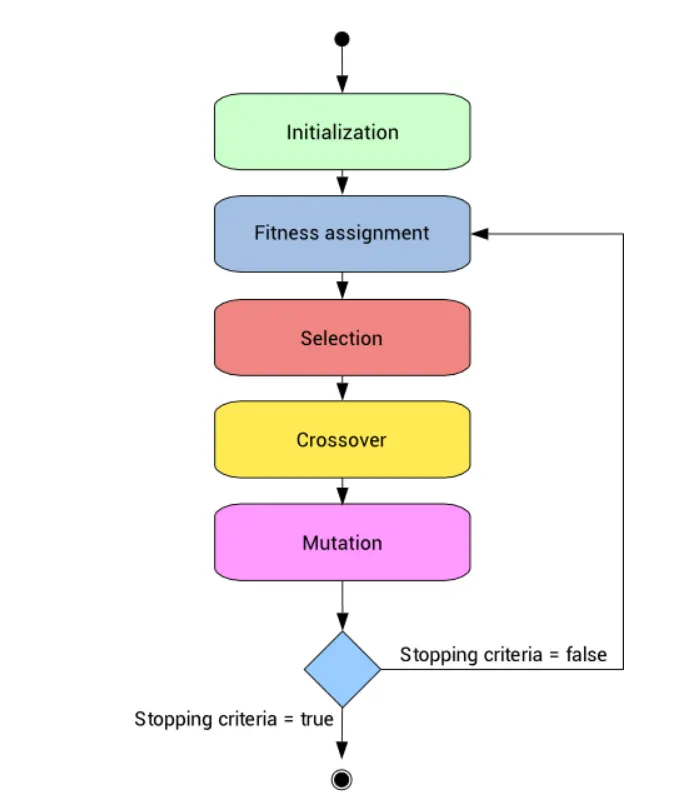
A FLOW CHART SHOWING HOW GA WORKS

EXPLAINATION OF SYNTAX OF ga (GENETIC ALGORITHM)

[x, fval, exitflag, output, population, scores ] = ga(fun, nvars, A, b, Aeq, beq, lu, ub, nonlcon, options)

fun = Function or fittness function.

nvars = Number of variables.

A, b = Linear inequalities Aeq*x = beq andA*x,<=b (set A = [] if non linear inequalities exists ga evaluates th matrix product Aeq*x as if x is transposed Aeq*x').

lb = Lower Bound.

up = upper bounds.

nonlcon = subjects the minimization to constraints define in the nonlcon. The function nonlcon accepts x and returns vector C and Ceq, representating the non linear inequalities and equalities respectively. ga minimizes the function such that C(x) <= 0 and Ceq(x) = 0.

options = minimizes with the default optimization parameters replaced by value in option.

x = Optimum soltuion or finds the minimum for the problem.

fval = The value of fitness function at x.

exitflag = An integer identifying the reason the algorithm terminated, and output, a structure that contains from each generation and other information about the performance of the algorithm.

population - Returns a matrix population, whose rows are final populatiion.

scores = Score of the final population.

STALAGMITE FUNCTION

The word stalagmite is purely geograpich, it is pointing cone like structure that grow inside caves due to mineral deposition. Stalagmite grow from the floor of the cave and stalacite grow from the celing of the cave.

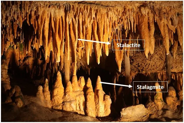
The main objective of stalagmite function is to generate these stalagmite and stalacite surfaces to represent data and to find out local and global maxima of that particular given function.

Given Below Is The Image Of Mathematical Formulation Of Stalagmite Function

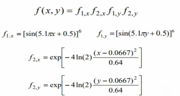
MATLAB code for Stalagmite function is given below which will be used in other part of the MATLAB program for optimization purpose. It is fittness function over here. THE EXPLAINATION ABOUT THE CODE IS GIVEN INSIDE THE CODE BODY.

function  [f] = stalagmite(input_vector)

x = input_vector(1);
y = input_vector(2);

f1_x = (sin(5.1*pi*x +0.5)).^6;
f1_y = (sin(5.1*pi*y +0.5)).^6;

a = ((x - 0.0667).^2)/(0.64);
f2_x = exp(-4.*log(2)*a);

b = ((y - 0.0667).^2)/(0.64);
f2_y = exp(-4.*log(2)*b);

f = -(f1_x.*f2_x.*f1_y.*f2_y);
end

• -ve sign in f is used so that we can find maxima of the given function using ga optimization, as ga gives minima of function by default.

CODE FOR OPTIMIZATION OF STALAGMITE FUNCTION AND TO FIND GLOBAL MAXIMA ALONG WITH 3 CASE STUDY AND THERIR RESULTS AND PLOT IS GIVEN BELOW.

clear all 
close all
clc

% Defining our search space
x = linspace(0,0.6,150);
y = linspace(0,0.6,150);


% Creating 2-dimensional mesh using meshgrid command for the above x and y

[xx yy] = meshgrid(x,y);
num_case = 50

% Evaluating stalagmite function using loop,for each value of x and y an
% array is created called input vector, it is a row vectoritt has 2
% coloumn. Stalagmite takes the input vector and calculates f. These 2
% loops are generating a plot for the given data.

for i = 1:length(xx)
    for j = 1:length(yy)
        input_vector(1) = xx(i,j);
        input_vector(2) = yy(i,j);
        f(i,j) = stalagmite(input_vector);
    end
end
% surfc command generates a smooth stalagmite surface for the calculation
% of global minima and maxima.

surfc(xx,yy,-f)

% shading interp removes the grid line from the surface of stalagmite.

shading interp

% Applying genetic algorithm to get maximum of the given function,we get
% the optimum value of x and y and it also gives the function value at optimum points.

[x,fval] = ga(@stalagmite,2)

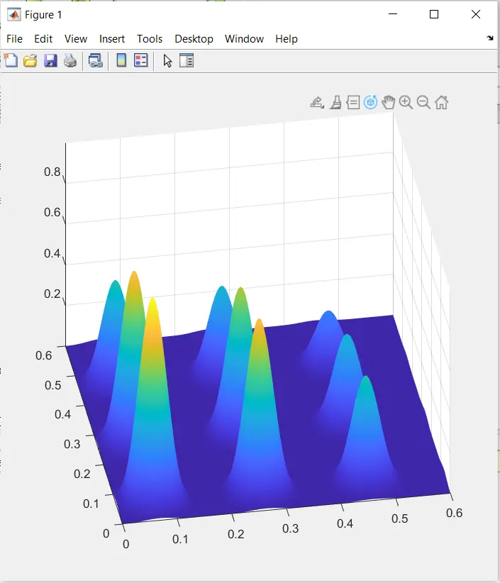
The below image is the result of the above code.

• Study 1 - Statistical Study Code Along With Explianation.

clear all
close all
clc
x = linspace(0,0.6,150);
y = linspace(0,0.6,150);
num_cases = 50

% Creating 2-dimensional mesh using meshgrid command for the above x and y.

[xx yy] = meshgrid(x,y);
num_case = 50

% Evaluating stalagmite function using loop,for each value of x and y an
% array is created called input vector, it is a row vectoritt has 2
% coloumn. Stalagmite takes the input vector and calculates f. These 2
% loops are generating a plot for the given data.



for i = 1:length(xx)
    for j = 1:length(yy)
        input_vector(1) = xx(i,j);
        input_vector(2) = yy(i,j);
        f(i,j) = stalagmite(input_vector);
    end
end


% Study 1 statistical behaviour, overhere the ga is called. The loop stores
% the value of x and y and alos the optimum values that function predicts.

tic
for i = 1:num_cases
    [input,fopt(i)] = ga(@stalagmite,2);
    xopt(i) = input(1);
    yopt(i) = input(2);
end
study1_time = toc

% A new figure window is opened. 

figure(1)
% Subplot command is used to create multiple plots in same window.
subplot(2,1,1)
hold on
% Plotting stalagmite function.
surfc(x,y,-f)
shading interp

% plot3 command is used to plot the 2nd loop in the same stalagmite plot
% to represent the results obtained over the 50 studies. It helps to
% visualize how the algorithm is functioning.

plot3(xopt,yopt,-fopt,'marker','o','markersize',5,'markerfacecolor','r')
title('unbounded inputs')

% The 2nd subplot directly plots the optimum values that the function
% predicts as the function of iterations which is basically the case number
subplot(2,1,2)
plot(-fopt)
xlabel('Iterations')
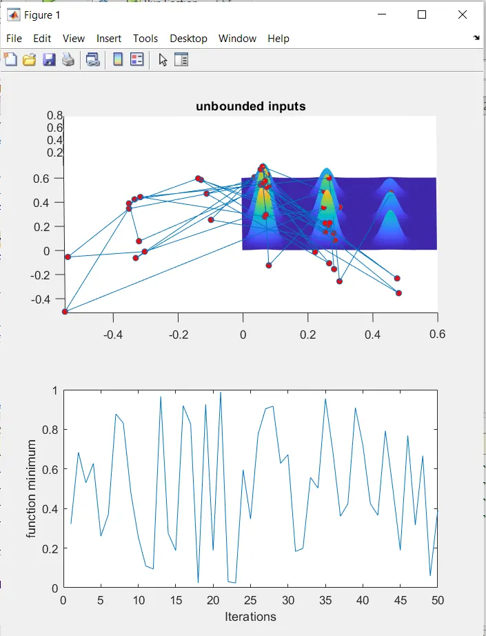
ylabel('function minimum')

• Results from the above code.

• Study 2 Statistical Behaviour With Upper And Lower Bounds. Given below is the code for the same along with proper explaination inside the code.

clear all
close all
clc
x = linspace(0,0.6,150);
y = linspace(0,0.6,150);
num_cases = 50

[xx yy] = meshgrid(x,y);
num_case = 50

% Evaluating stalagmite function

for i = 1:length(xx)
    for j = 1:length(yy)
        input_vector(1) = xx(i,j);
        input_vector(2) = yy(i,j);
        f(i,j) = stalagmite(input_vector);
    end
end


% Study 2 statisctical behaviour with upper and lower bounds, overhere the
% bounds are sey to stop x and y ffrom going below 0 and above 0.6, rest
% all the code is like study 1.

tic
for i = 1:num_cases
    [input,fopt(i)] = ga(@stalagmite,2,[],[],[],[],[0,0],[1,1]);
    xopt(i) = input(1);
    yopt(i) = input(2);
end
study1_time = toc

figure(1)
subplot(2,1,1)
hold on
surfc(x,y,-f)
shading interp
plot3(xopt,yopt,-fopt,'marker','o','markersize',5,'markerfacecolor','r')
title('Bounded inputs')
subplot(2,1,2)
plot(-fopt)
xlabel('Iterations')
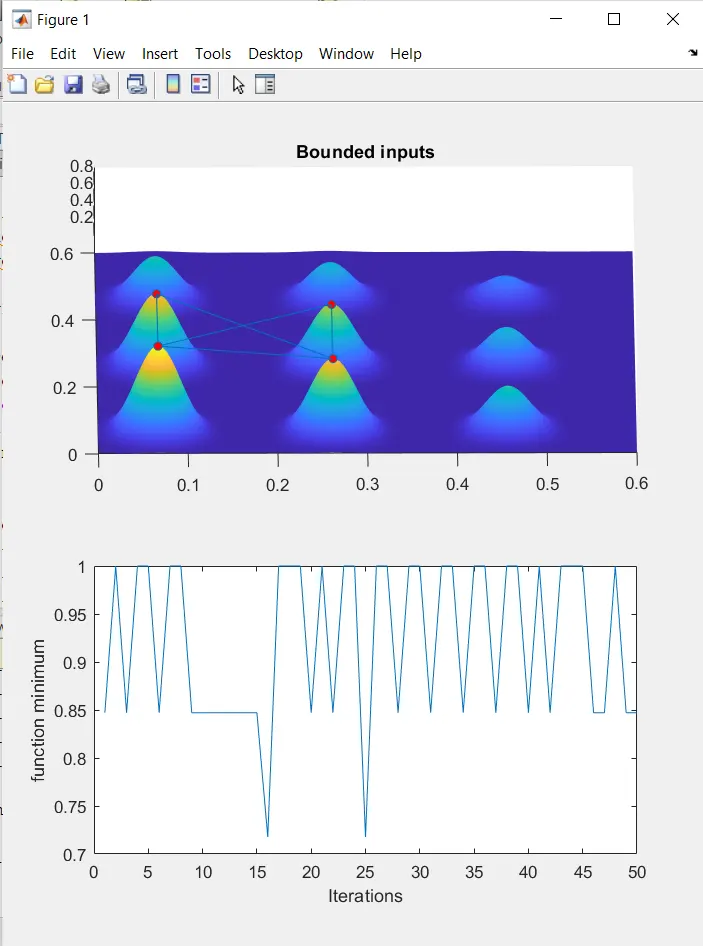
ylabel('function minimum')

• Results for the above code is given below.

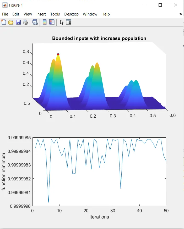
• Study 3 along with bounds population size is increased. Below is the MATLAB code along with explaination.

clear all
close all
clc
x = linspace(0,0.6,150);
y = linspace(0,0.6,150);
num_cases = 50

[xx yy] = meshgrid(x,y);
num_case = 50

% Evaluating stalagmite function

for i = 1:length(xx)
    for j = 1:length(yy)
        input_vector(1) = xx(i,j);
        input_vector(2) = yy(i,j);
        f(i,j) = stalagmite(input_vector);
    end
end


% Study 3 increasing ga iterations, over here along with boundation
% initial population size is also increased. If the initial populaion size
% is too small than it cannot find global maxima but local maxima. To
% ovrcome this population size increased to 300. The disadvantage of thiis
% is that it will slow down the ga because of more number of samples and
% individuals.

options = optimoptions('ga');
options = optimoptions(options,'populationsize',300);

tic
for i = 1:num_cases
    [input,fopt(i)] = ga(@stalagmite,2,[],[],[],[],[0,0],[1,1],[],[],options);
    xopt(i) = input(1);
    yopt(i) = input(2);
end
study1_time = toc

figure(1)
subplot(2,1,1)
hold on
surfc(x,y,-f)
shading interp
plot3(xopt,yopt,-fopt,'marker','o','markersize',5,'markerfacecolor','r')
title('Bounded inputs with increase population')
subplot(2,1,2)
plot(-fopt)
xlabel('Iterations')
ylabel('function minimum')

• Given below is the results obtained from the above code.