Project 1 - Parsing NASA thermodynamic data

AIM

To write a MATLAB program to extract 14 co-efficients for each species from NASA THERMO.dat file and calculate there specific heat, entropy and enthalpy. We also have to plot (T,s), (T,h) & (T,cp) for every species and at the same time calculate the molecular mass for all species.

FILE PARSING

It is a method of extracting data from a file. The code must have some generalised rule or synatx so that it can fetch data from different kind of files where the data is arranged in different manner.

Over here we are extracting 14 co-efficients from the NASA THERMO.dat which will be feeded to the NASA'S polynomial to find the properties of 53 elements or compound species by calculating there entropy, enthalpy and specific heat. The first 7 co-efficients are Local High Temperature and then the following second are Low Temperature co-efficients.

R = Uniiversal Gas Constant.

T = Temperature.

NASA'S POLYNOMIALS WHICH WILL BE USED HERE.

PROGRAM LOGIC EXPLAINATION

1. The THERMO.dat file is imported by using fopen command and then all other lines are read by using fgetl command.
2. Header information is fetched by using fgetl command and then strsplit command is used to split the string using delimiters which is on next part is store to different variables by converting them into number by using str2num command.
3. Next 3 lines are comments and hence they are skipped, as it is cleared from the code.
4. Species data is read and since 53 species are there so the logic to extract each spesies data remains the same hence for loop is used.
5. In speciess section the first line contains species name and Local Temperature Range followed by 3 lines which contain 14 co-efficients.
6. Again the strsplit command is used to split the first line and get the species_name and Local Temperature Range.
7. To get the 14 co-efficient strfind comand is used to find the location of 'E', in command window it will return numbers where these 'E' are located in that line using that results 14 co-efficients are found. It is clearly understandable from code.
8. str2num command is used to convert the strings type co-efficients obtained in last step to number which can be used in further calculation.
9. For plotting we need a range of temperature so Local Temperature Range is splitted into 1000 points using linspace commands.
10. For loop is used to decide whether to feed high temperature range or low temperature range into the NASA polynomials by comparing it with Medium Local Temperature point over 1000 range of temperature points which will also be feeded into polynomial.
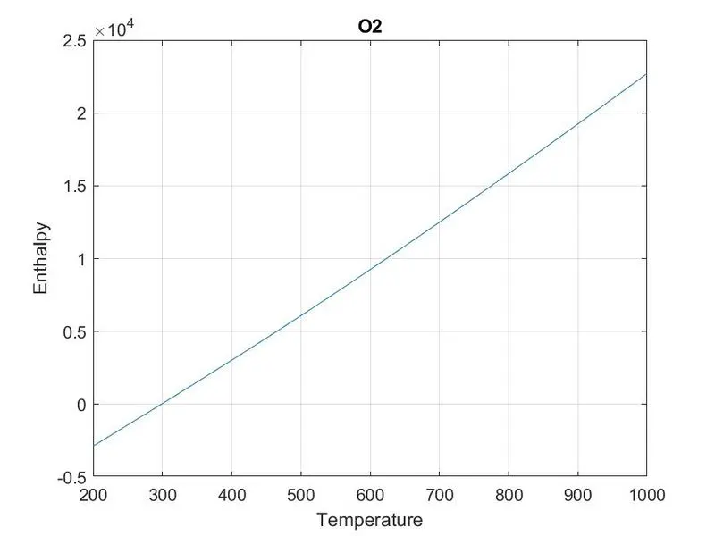
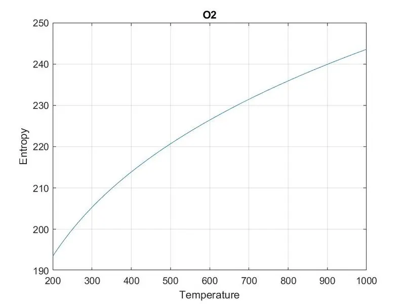
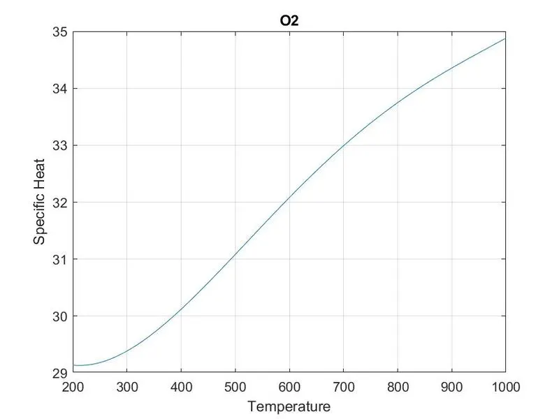
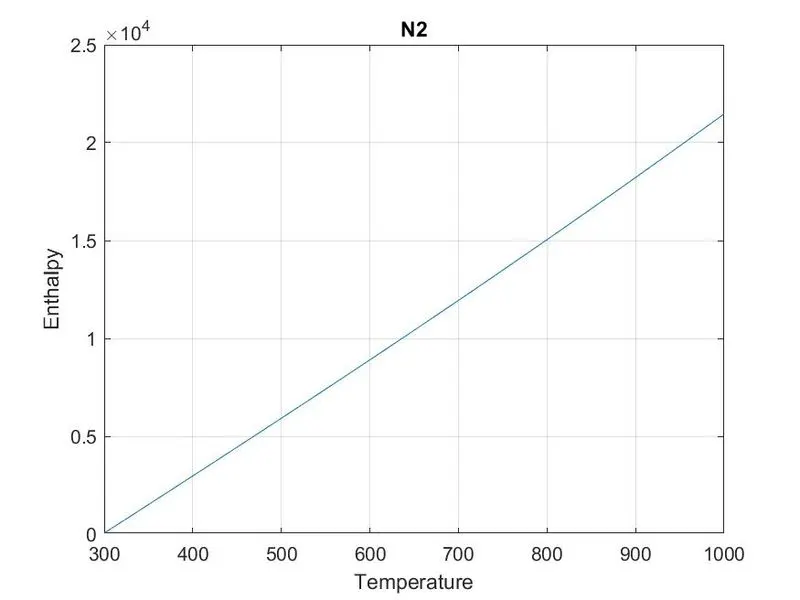
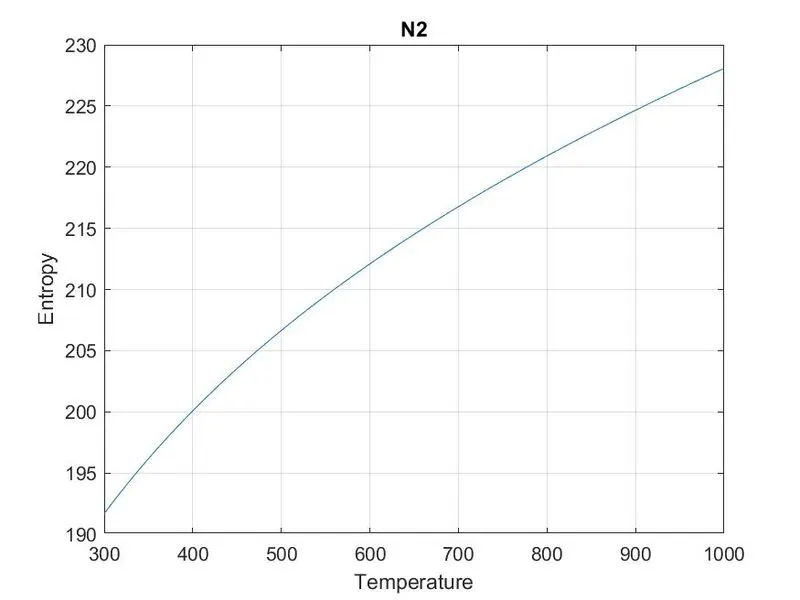
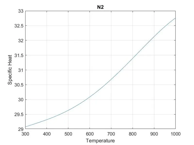
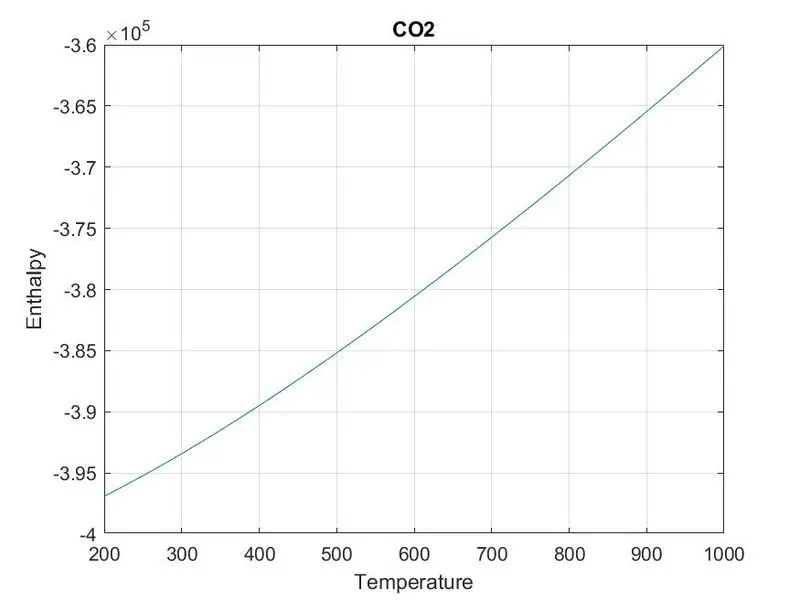
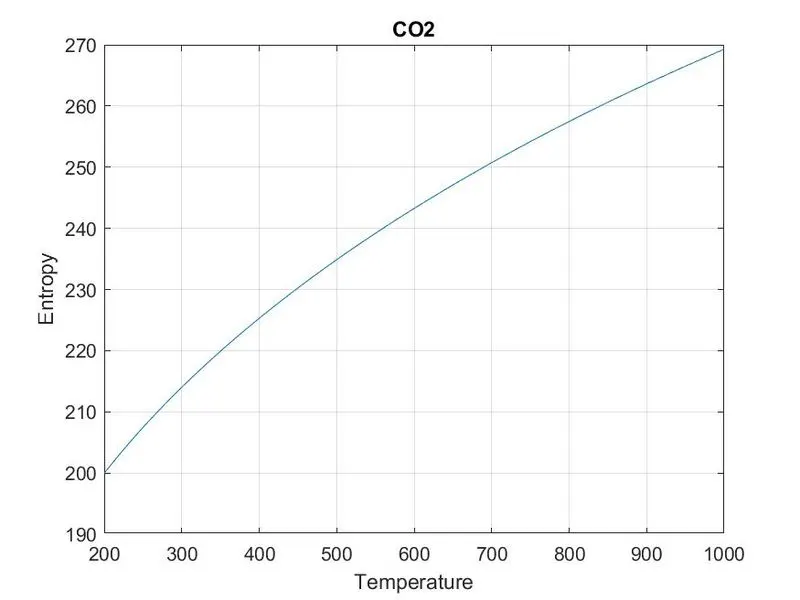
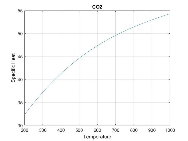
11. Plotting is done for (T,s), (T,h) & (T,cp) using the plot command.
12. For saving the file cd command is used along with saveas command.
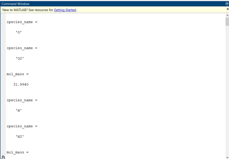
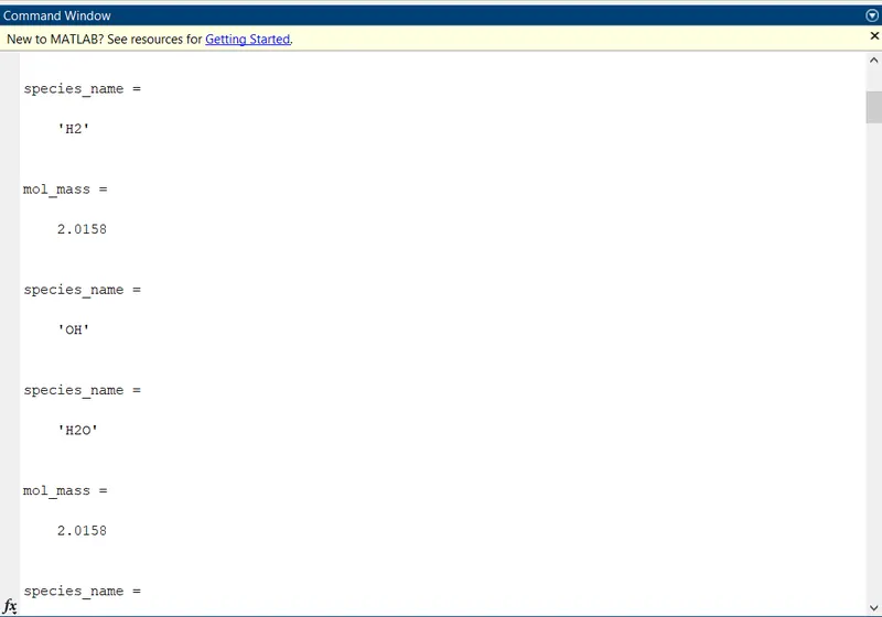
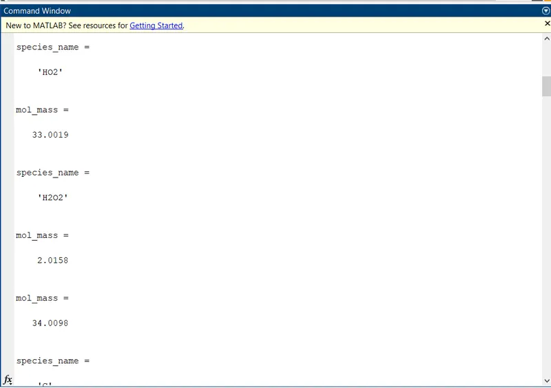
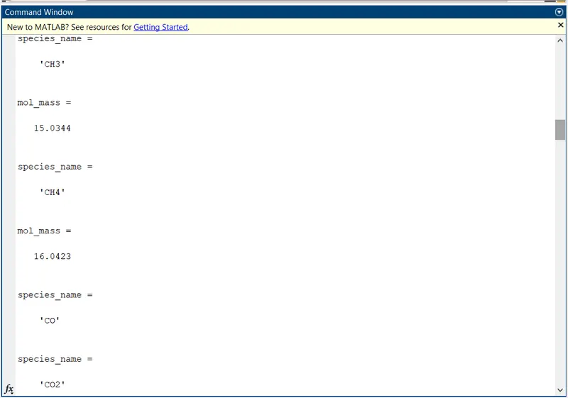
13. Atomic weight is assigned to each elements and the molecular mass is calculated using by 2 for loops. One to iterate species_name elements and second loop compares the elements with the species element using the if statement and if it is true then the coresponding number atomic_weight is added to Molecular mass and the same number is use to store the position position of element by using flag operator q = p, q is use as flag operator it stores the position of that particular element for next if condition which will calculate the atomic number in case that element is present more than 1 time in the species like CO2 or H2O etc.

MAIN FILE PARSING CODE

clear all
close all
clc

% Opening Nasa's file
f1 = fopen('THERMO.dat','r');
first_line = fgetl(f1);

% Defining the global maximum, medium and minimum tempertures
global_temp = fgetl(f1);
A = strsplit(global_temp,' ');
global_min_temp = str2num(A{2});
global_med_temp = str2num(A{3});
global_max_temp = str2num(A{4});

% Skipping the comments
comment_1 = fgetl(f1);
comment_2= fgetl(f1);
comment_3 = fgetl(f1);

% Getting the coefficient of species.
for i=1:53
% Extracting line 1 the name of the species.
header = fgetl(f1);
line_1 = strsplit(header,' ');
species_name = (line_1{1})
z = length(line_1);
local_low_temp = str2num(line_1{z-3});
local_medium_temp = str2num(line_1{z-2});
local_high_temp = str2num(line_1{z-1});

% Extracting Higer And Lower Temperatures Coefficients.

line2 = fgetl(f1);
line3 = fgetl(f1);
line4 = fgetl(f1);


A = strfind(line2,'E');
B = strfind(line3,'E');
C = strfind(line4,'E');

% Extracting Higer Temperature Coefficients.
a1 = str2num(line2(1:A(1)+3));
a2 = str2num(line2(A(1)+4:A(2)+3));
a3 = str2num(line2(A(2)+4:A(3)+3));
a4 = str2num(line2(A(3)+4:A(4)+3));
a5 = str2num(line2(A(4)+4:A(5)+3));
a6 = str2num(line3(1:B(1)+3));
a7 = str2num(line3(B(1)+4:B(2)+3));

%Extracting Lower Temperature Coefficients.
b1 = str2num(line3(B(2)+4:B(3)+3));
b2 = str2num(line3(B(3)+4:B(4)+3));
b3 = str2num(line3(B(4)+4:B(5)+3));
b4 = str2num(line4(1:C(1)+3));
b5 = str2num(line4(C(1)+4:C(2)+3));
b6 = str2num(line4(C(2)+4:C(3)+3));
b7 = str2num(line4(C(3)+4:C(4)+3));

T = linspace(local_low_temp,local_high_temp,1000);
R = 8.314;

% To get the array of specific heat(cp), entropy (s) & enthalpy (h)

for k = 1:length(T)
    %Below if statement is use to assign higher or lower temperature
    %coefficients.
    if T(k)>local_medium_temp
        % Higher Temperature Coefficient is used.
        
        cp(k) = R.*(a1+(a2.*T(k))+(a3.*T(k).^2)+(a4.*T(k).^3)+(a5.*T(k).^4));
        
        s(k) = R*(a1.*log(T(k))+a2.*T(k)+(a3.*T(k).^2)/2+(a4.*T(k).^3)/3+(a5.*T(k).^4)/4+a7);
        
        h(k)= R.*(a1.*T(k)+(a2.*T(k).^2)/2+(a3.*T(k)^3)/3+(a4.*T(k).^4)/4+(a5.*T(k).^5)/5+a6);
        
    else
        % Lower Temperature coefficient is used.
        
        cp(k) = R.*(b1+(b2.*T(k))+(b3.*T(k).^2)+(b4.*T(k).^3)+(b5.*T(k).^4));
        
         s(k) = R*(b1.*log(T(k))+(b2.*T(k))+(b3.*T(k).^2)/2+(b4.*T(k).^3)/3+(b5.*T(k).^4)/4+b7);
         
          h(k) = R.*(b1.*T(k)+(b2.*T(k).^2)/2+(b3.*T(k).^3)/3+(b4.*T(k).^4)/4+(b5.*T(k).^5)/5+b6);
    end
end


% Plotting the graphs for (T,s), (T,h) and (T,cp)

figure(1)
plot(T,cp);
title(species_name)
xlabel('Temperature')
ylabel('Specific Heat')
grid on;

figure(2)
plot(T,s);
title(species_name)
xlabel('Temperature')
ylabel('Entropy')
grid on;

figure(3)
plot(T,h);
title(species_name)
xlabel('Temperature')
ylabel('Enthalpy')
grid on;

% Changing the directory and saving the file
mkdir(['C:\MATLAB\File Parsing Results\',species_name]);
cd(['C:\MATLAB\File Parsing Results\',species_name]);

saveas(figure(1),'Specific Heat','jpg');
saveas(figure(2),'Entropy','jpg');
saveas(figure(3),'Enthalpy','jpg');


% Calculating Molecular Mass of the Species 

elements = ['H','C','O','N','A'];
atomic_weight = [1.0079 12.0107 15.997 14.0067 39.948];
mol_mass = 0;

for o = 1:length(species_name)
    for p = 1:length(elements)
        if strcmp(species_name(o),elements(p))
            mol_mass = (mol_mass + atomic_weight(p));
            q = p;
        end
    end

    n = str2num(species_name(o));
    if n>1
        mol_mass = mol_mass + (atomic_weight(q)*(n-1))
    end
end

end

fclose(f1)
        


        
        

RESULTS FROM THE ABOVE CODE

• PLOTS FOR O2

• PLOTS FOR N2

• PLOTS FOR CO2

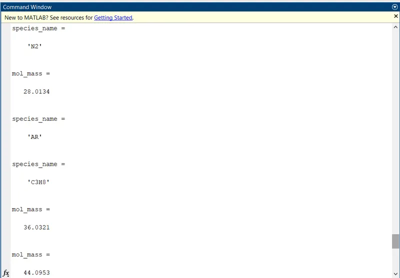
• MOLECULAR MASS OF SPECIES