Week 4.1 - Genetic Algorithm

AIM - To write a code to optimize the stalagmite function and find the function's global maxima using a genetic algorithm.

GOVERNING EQUATION - The stalagmite function for the genetic algorithm of global minima is shown below:

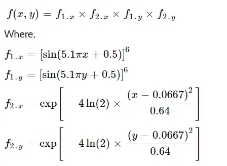
now as mentioned the above equations are for finding the global minima but I have to find the global maxima for that I have to use the negative sign before the equation. so the equation for finding the global maxima will be:

OBJECTIVE - 1) To optimize the stalagmite function and to find the global maxima of the function.

2) To explain the concept of genetic algorithms and also the syntax for ga in Matlab.

3) To plot the graphs for all the study done for the optimization process.

THEORY - Genetic Algorithm - The genetic algorithm is a method for solving both constrained and unconstrained optimization problems that are based on natural selection, the process that drives biological evolution. The genetic algorithm repeatedly modifies a population of individual solutions. At each step, the genetic algorithm selects individuals at random from the current population to be parents and uses them to produce the children for the next generation. Over successive generations, the population "evolves" toward an optimal solution. You can apply the genetic algorithm to solve a variety of optimization problems that are not well suited for standard optimization algorithms, including problems in which the objective function is discontinuous, nondifferentiable, stochastic, or highly nonlinear.

A brief overview of the genetic algorithm is mentioned below:

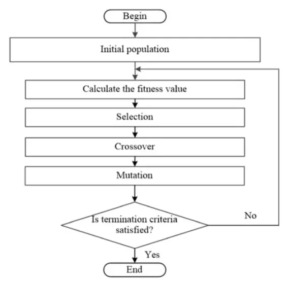
Five phases are considered in a genetic algorithm.

1. Initial population - The process begins with a set of individuals which is called a Population. Each individual is a solution to the problem you want to solve.An individual is characterized by a set of parameters (variables) known as Genes. Genes are joined into a string to form a Chromosome (solution).In a genetic algorithm, the set of genes of an individual is represented using a string, in terms of an alphabet. Usually, binary values are used (strings of 1s and 0s). We say that we encode the genes in a chromosome.

2. Fitness Function - The fitness function determines how fit an individual is (the ability of an individual to compete with other individuals). It gives a fitness score to each individual. The probability that an individual will be selected for reproduction is based on its fitness score.

3. Selection - The idea of the selection phase is to select the fittest individuals and let them pass their genes to the next generation. Two pairs of individuals (parents) are selected based on their fitness scores. Individuals with high fitness have more chances to be selected for reproduction.

4. Crossover - Crossover is the most significant phase in a genetic algorithm. For each pair of parents to be mated, a crossover point is chosen at random from within the genes. In the crossover, Offspring is created by exchanging the genes of parents among themselves until the crossover point is reached and then they are added to the population.

5. Mutation - In certain new offspring formed, some of their genes can be subjected to a mutation with a low random probability. This implies that some of the bits in the bit string can be flipped. Mutation occurs to maintain diversity within the population and prevent premature convergence.

some of the applications of Genetic algorithms are as follows:

• Vehicle routing problems
• Scheduling applications
• DNA Analysis
• Robot Trajectory Generation
• Parametric Design of Aircraft

now let see what is stalagmite function

Stalagmite Function - Stalagmite functions are the mathematical model that helps us generate local maxima and minima or the global maxima or minima. This function is called stalagmite because the output looks like a stalagmite. A stalagmite is a type of rock formation that rises from the floor of a cave due to the accumulation of material deposited on the floor from ceiling drippings.

PROGRAM - Here first I have to create the program for the stalagmite function which I will use in my main program. The program for stalagmite function is shown below:

% program for writing the function
function [f] = stalagmite(input_vector)
x = input_vector(1);
y = input_vector(2);

f1 = (sin(5.1*pi*x + 0.5).^6);
f2 = (sin(5.1*pi*y + 0.5).^6);
f3 = exp(-4*log(2)*(((x-0.0667).^2)/0.64));
f4 =  exp(-4*log(2)*(((y-0.0667).^2)/0.64));

f = -(f1*f2*f3*f4);
end

In the above program, the function command is used to create a template of the stalagmite function so that it can be used whenever we want. For this program function, the stalagmite is the name of the function which I will be writing to call the program and input_vector is the inputs that I will be giving. so x and y are two inputs for this function and then I have written the equation:

I have assigned separate terms for each equation and then multiplied all the terms to get the final function. And as mentioned I have to find the global maxima and the above equations are for finding the global minima so I have to use the negative sign(-) to find the global maxima so that is what I have done.

Now I have written the main program in which I will use the above function to get the output using a genetic algorithm. The main program is shown below:

clear all
close all
clc

x = linspace(0,0.6,100);
y = linspace(0,0.6,100);
% creating two dimensional arrays
[xx yy] = meshgrid(x,y);

for i = 1:length(xx)
    for j = 1:length(yy)
        input_vector(1) = xx(i,j);
        input_vector(2) = yy(i,j);
        f(i,j) = stalagmite(input_vector);
    end
end
% plotting the surface
surfc(xx,yy,f)
shading interp

[inputs,fval] = ga(@stalagmite,2)
xlabel('x axis')
ylabel('y axis')
legend('x values','y values')
title('stalagmite function')

num_cases = 50;


   
%study 1 statistical behaviour
  tic
for i = 1: num_cases
    [inputs,fopt(i)] = ga(@stalagmite,2);
    xopt(i) = inputs(1);
    yopt(i) = inputs(2);
end
  toc
figure(2)
subplot(2,1,1)
hold on
surfc(x,y,f)
shading interp
plot3(xopt,yopt,fopt,'marker','o','markersize',10,'markerfacecolor','b');
title('unbound inputs')
subplot(2,1,2)
plot(fopt)
xlabel('Iterations')
ylabel('Function maxima')

% study 2 statistical behaviour with upper and lower bounds
 tic
for i = 1:num_cases
    [inputs,fopt2(i)] = ga(@stalagmite,2,[],[],[],[],[0;0],[1;1]);
    xopt(i) = inputs(1);
    yopt(i) = inputs(2);
end
 toc
figure(3)
subplot(2,1,1)
hold on
surfc(x,y,f)
shading interp
plot3(xopt,yopt,fopt2,'marker','o','markersize',10,'markerfacecolor','b');
title('bounded inputs')
subplot(2,1,2)
plot(fopt2)
xlabel('Iterations')
ylabel('Function maxima')

% study 3 statistical behaviour with upper and lower bounds and population
options = optimoptions('ga');
options = optimoptions(options,'populationsize',300);
  study_time = tic
for i = 1 : num_cases
    [inputs,fopt3(i)] = ga(@stalagmite,2,[],[],[],[],[0;0],[1;1],[],[],options);
    xopt(i) = inputs(1);
    yopt(i) = inputs(2);
end
study_time = toc
figure(4)
subplot(2,1,1)
hold on
surfc(x,y,f)
shading interp
plot3(xopt,yopt,fopt3,'marker','o','markersize',10,'markerfacecolor','b');
title('bounded inputs with population')
subplot(2,1,2)
plot(fopt3)
xlabel('Iterations')
ylabel('Function maxima')

Now first I have written the program for solving the stalagmite function using a genetic algorithm. The program is shown below:

clear all
close all
clc

x = linspace(0,0.6,100);
y = linspace(0,0.6,100);
% creating two dimensional arrays
[xx yy] = meshgrid(x,y);

for i = 1:length(xx)
    for j = 1:length(yy)
        input_vector(1) = xx(i,j);
        input_vector(2) = yy(i,j);
        f(i,j) = stalagmite(input_vector);
    end
end
% plotting the surface
surfc(xx,yy,f)
shading interp

[inputs,fval] = ga(@stalagmite,2)
xlabel('x axis')
ylabel('y axis')
legend('x values','y values')
title('stalagmite function')

In the above program, the clear all command will delete the data from the previously performed operation, close all command will close all the graphs or scope related to the previously performed operation. clc command will clear the command window.

Then I know that x and y are my two variables for the function so I have used the linspace command to get different values of x and y which will act as the input. In the program, linsapce command will create 100 different values of x andy between o to 0.6. Then to create the two-dimensional I have used the mesh grid command.

Now since I have to run the program for all values of x and y I have used the 'for' loop command which will make sure that all values of x and y are taken as input for ga. Here you can see 2 'for' loops are used. one for x and the other for y the inputs I have given are the mesh grid [xx and yy]. Then I have called the stalagmite which I created earlier. Next, I have ended both the 'for' loops.

Then I have used the surface command which makes a 3-dimensional plot of the output. So it will make a surface using (xx, yy,f). The shading interp command is used to remove lines and provides shade to the surface so as to see the output clearly.

Then I have used the genetic algorithm to solve the function. The ga command will take the inputs given and calculate the fval for the function. The ga is written as x= ga(fun,nvars) finds a local unconstrained minimum,x, to the objective function, fun.nvars is the dimension (number of design variables) of fun. so in my program, the functions stalagmite and the no. of variables (nvars) is 2 so that is what I have written. [x,fval] = ga(_) , for any previous input arguments, also returns fval, the value of the fitness function at x. In the program, x is replaced by input.

Then I have defined the x and y-axis using the label command. and I have also defined the legend. legend creates a legend with descriptive labels for each plotted data series. For the labels, the legend uses the text from the Displayname properties of the data series. Then at last I have the title to the output. After this next comes the optimization part.

Optimization - Optimization is a decision-making process it helps to find the best results under a set of prioritized criteria or constraints. It is a procedure that is executed iteratively by comparing various solutions till an optimum solution is found. so for the optimization process, I have done 3 studies. Study 1 is shown below:

  tic
for i = 1: num_cases
    [inputs,fopt(i)] = ga(@stalagmite,2);
    xopt(i) = inputs(1);
    yopt(i) = inputs(2);
end
  toc
figure(2)
subplot(2,1,1)
hold on
surfc(x,y,f)
shading interp
plot3(xopt,yopt,fopt,'marker','o','markersize',10,'markerfacecolor','b');
title('unbound inputs')
subplot(2,1,2)
plot(fopt)
xlabel('Iterations')
ylabel('Function maxima')

In the above study, I have just run the program giving the num_cases only the num_cases. The num_cases represents the time for which the genetic algorithm is made to run. In the program, it was 50. so in the first study, I have not defined any bounds and population size and just solved the function.

In the program, 'tic' command will start the clock time for the function. Then because I have to run the program 50 times I have again used the 'for' loop used the similar ga as I used earlier calling the stalagmite function and defining the variables. Then I have ended the for loop and the 'toc' command will stop the clock time

subplot function will help to plot different plots in one single plot. The hold-on command is used again because I want the output in one figure. Then again I have used the surface command which will again create a 3 d plot of the output.

The shading interp command is used to remove lines and provides shade to the surface so as to see the output clearly.

The plot3 command will plot coordinates of (x,y,z) in 3 D space. the inputs I have plotted in the program are xopt,yopt and fopt, and opt here stands for optimization. Then I have also given a 'marker' command to show the points and also given face color to that marker. Then I have given the title to the plot as well and also I have given the x and y labels as iterations and function maxima respectively. This completes study 1

Now I have written the program for study 2. The study 2 program part shown below:

% study 2 statistical behaviour with upper and lower bounds
 tic
for i = 1:num_cases
    [inputs,fopt2(i)] = ga(@stalagmite,2,[],[],[],[],[0;0],[1;1]);
    xopt(i) = inputs(1);
    yopt(i) = inputs(2);
end
 toc
figure(3)
subplot(2,1,1)
hold on
surfc(x,y,f)
shading interp
plot3(xopt,yopt,fopt2,'marker','o','markersize',10,'markerfacecolor','b');
title('bounded inputs')
subplot(2,1,2)
plot(fopt2)
xlabel('Iterations')
ylabel('Function maxima')

In the above program again I have run the program for num_cases which is 50 but this time I have also defined the upper and lower bounds which basically are the upper and lower limits of x and y. The study starts with the 'tic' which starts the clock timer for the function and then the 'for' loop again I will give the inputs. The genetic algorithm function this time will be different as I have to define the upper and lower limits

Here I have used x= ga(fun,nvars,A,b,Aeq,beq) finds a local minimum x of fun, subject to the linear equalities Aeq*x = be and A*x_x is transposed (Aeq*x').

x = ga(fun,nvars,A,b,Aeq,beq,lb,ub) defines a set of lower and upper bounds on the design variables x so that a solution is found in the range lb<x<ub. (Set Aeq = [] and beq = []if no linear equalities exist.) Here lb is lower bound and ub is upper bound.

In the program, I have called the stalagmite function so that is fun and nvars are 2. Here I don't have any linear inequality constraints so I have just left those places using [] brackets and then I have given the bounds so my lower bounds of x and y are (0,0) and the upper bounds of x and y are (1,1). The results from the genetic algorithm are stored in xopt and yopt and then i have ended the 'for' loop. and used the toc command to stop the clock. now the rest program lines are similar to study 1.

subplot function will help to plot different plots in one single plot. The hold-on command is used again because I want the output in one figure. Then again I have used the surface command which will again create a 3 d plot of the output.

The shading interp command is used to remove lines and provides shade to the surface so as to see the output clearly.

The plot3 command will plot coordinates of (x,y,z) in 3 D space. the inputs I have plotted in the program are xopt,yopt and fopt2, and opt here stands for optimization. Then I have also given a 'marker' command to show the points and also given face color to that marker. Then I have given the title to the plot as well and also I have given the x and y labels as iterations and function maxima respectively. This completes study 2.

Now the study 3 program part is shown below:

% study 3 statistical behaviour with upper and lower bounds and population
options = optimoptions('ga');
options = optimoptions(options,'populationsize',300);
  study_time = tic
for i = 1 : num_cases
    [inputs,fopt3(i)] = ga(@stalagmite,2,[],[],[],[],[0;0],[1;1],[],[],options);
    xopt(i) = inputs(1);
    yopt(i) = inputs(2);
end
study_time = toc
figure(4)
subplot(2,1,1)
hold on
surfc(x,y,f)
shading interp
plot3(xopt,yopt,fopt3,'marker','o','markersize',10,'markerfacecolor','b');
title('bounded inputs with population')
subplot(2,1,2)
plot(fopt3)
xlabel('Iterations')
ylabel('Function maxima')

In study 3 again I have run the model for mun_cases but this time along with the lower and upper bounds I have also defined the population size. The function will focus on that population size along with the bounds and calculate the output.

Here for providing the population size I have used the options command.

so the line options = optimoptions('ga') will return default options for the solver name. Then the next line options = optimoptions(options,'populationsize',300) returns a copy of options with the named parameters altered with the specific values. The population size I have assigned was 300.

Then again the similar thing 'tic' command for starting the clock then again the for loop for running the program 50 times. Then for calculating the optimum value the syntax for ga I have used was: x=ga(fun,nvars,A,b,Aeq,beq,lb,ub,non1con,intcon,optioms) minimizes with the default optimization parameters replaced by values options.

here the new terms are non1con and intcon which are nonlinear constrains and integer constraints but in my program, I have not considered that so I have used the [] brackets to fill the place. The results from the genetic algorithm are stored in xopt and yopt then i have ended the 'for' loop. and used the toc command to stop the clock. now the rest program lines are similar to study 2.

subplot function will help to plot different plots in one single plot. The hold-on command is used again because I want the output in one figure. Then again I have used the surface command which will again create a 3 d plot of the output for (x,y,f)

The shading interp command is used to remove lines and provides shade to the surface so as to see the output clearly.

The plot3 command will plot coordinates of (x,y,z) in 3 D space. the inputs I have plotted in the program are xopt,yopt and fopt3, and opt here stands for optimization. Then I have also given a 'marker' command to show the points and also given face color to that marker. Then I have given the title to the plot as well and also I have given the x and y labels as iterations and function maxima respectively. This completes study 3 and also the program.

RESULT - The plot for the solution of stalagmite function is shown below:

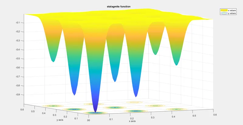
Now for the above-shown stalagmite, I have optimized the function by multiple studies to find the global maxima coordinates. The output of study one which is just running the function 50 times giving the inputs is shown below:

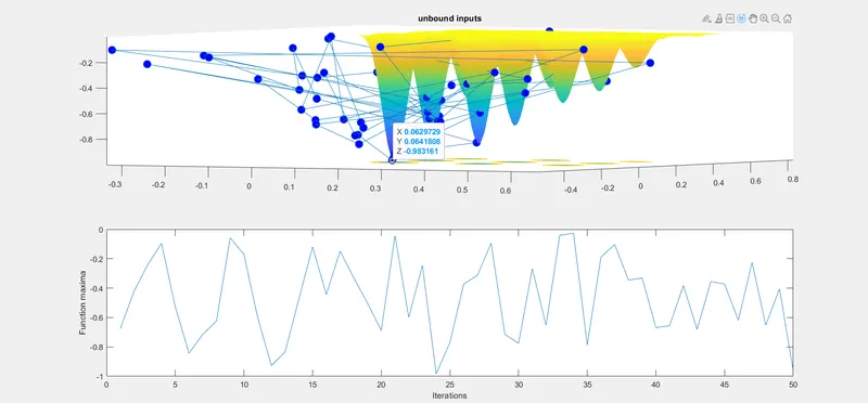
so in the above output, we can see that the blue dots which are for the global maxima calculation are scattered randomly and it does not look good. so in order to solve this issue, I have done the study 2 which consist of lower and upper bounds so the result of study 2 is shown below:

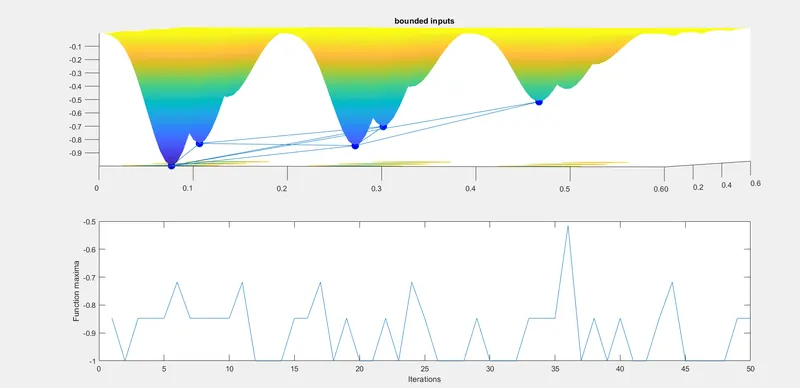
Now the above plot looks better but still, it has a lot of blue dots or we can say that those are local maxima so for finding the global maxima i have done study 3 which includes lower and upper bounds along with the population size of 300. so the result of study 3 is shown below:

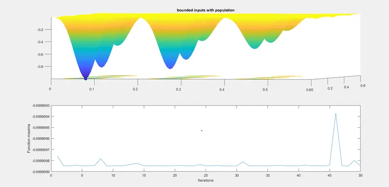
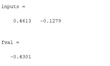
Here we can see that there is only one blue dot and that is the global maxima for the stalagmite function. The time took to find the global maxima was 17.1564 seconds.

The fval for the function along with the coordinates of global maxima is shown below:

CONCLUSION - The program to optimize the stalagmite function and find the function's global maxima using a genetic algorithm has been completed successfully and the results are shown.