Week 4.1 - Genetic Algorithm

Analysis of a Stalagmite Function and Optimising it using the Genetic Algorithm with 3 case studies in MATLAB

Aim: To try and understand the concept of genetic algorithm by referring various sources, learn more about the stalagmite function, and the ways to optimise it using the Genetic Algorithm.

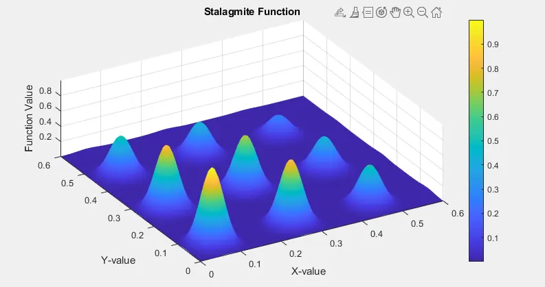
Stalagmite Function

1. To Write a code in MATLAB in order to optimize and find the global maxima of the stalagmite function.
2. To Explain the concepts of genetic algorithm and its syntaxes we have used here to optimisie stalagmite function using "ga" in MATLAB.
3. To Plot graphs for `F_(m a x im u m)` v/s no. of iterations for different case studies.

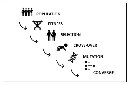
Theory: GENETIC ALGORITHM :- The genetic algorithm is a method for solving both constrained and unconstrained optimization problems that is based on natural selection, the process that drives biological evolution in short. The genetic algorithm repeatedly modifies a population of individual solutions. At each step, the genetic algorithm selects individuals at random from the current population to be parents and uses them to produce the children for the next generation. Over successive generations, the population "evolves" toward an optimal solution. You can apply the genetic algorithm to solve a variety of optimization problems that are not well suited for standard optimization algorithms, including problems in which the objective function is discontinuous, nondifferentiable, stochastic, or highly nonlinear. The genetic algorithm can address problems of mixed integer programming, where some components are restricted to be integer-valued. The various phases that GA undergoes during solving a problem are,

1. Initial Population
2. Fitness Function
3. Selection
4. Crossover
5. Mutation
6. Convergence

Optimization :- Optimization is a process which is used to find the best solution out of all possible solutions available. One such process is the Genetic Algorithm (GA) which is built on the basis of theory of evolution by Natural Selection proposed by Charles Robert Darwin in 1859.

Initial Population:- The process begins with the set of individual values which is called population. Each individual is a solution to the problem that has to be solved.

Fitness Function:- Fitness function determines how fit an individual is by providing a fitness score to the individual. Based on the fitness score the individuals will be selected for crossover.

Selection:- In selection process two individuals (parents) will be selected for reproduction based on the fitness score which is higher.

Crossover:- Crossover is the process where the selected fit individuals chooses a point to exchange their genes in order to produce the offsprings.

Mutation:- In the offsprings, the permanent alteration in the DNA sequence that makes up a gene in order to maintain diversity with the population and premature convergence is called Mutation.

Convergence:- Convergence is that the state at which the algorithm comes to an end i.e., when there is no improvement in the solution quantity or an acceptable solution is obtained.

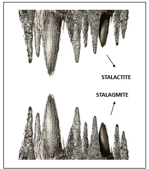
What is a Stalagmite?

A stalagmite is a type of rock formation that rises from the floor of a cave due to the accumulation of material deposited on the floor from ceiling drippings. Stalagmites are typically composed of calcium carbonate, but may consist of lava, mud, peat, pitch, sand, sinter and amberat.

Stalagmite Function :- The function that is used to obtain the 3D model of a stalagmite model is given as follows,

`f(x,y) = (f1_x*f2_x*f1_y*f2_y)`

Where,

`f1_x` = `[sin((5.1*π*x)+0.5)]^6`

`f2_x` = `exp[(-4*ln(2))*(((x-0.0667)^2)/0.64)]`

`f1_y` = `[sin((5.1*π*y)+0.5)]^6`

`f2_y` = `exp[(-4*ln(2))*(((y-0.0667)^2)/0.64)]`

Here 'x' and 'y' are going to be the inputs of the co-ordinates for which the global maximum and local maximum will be calculated.

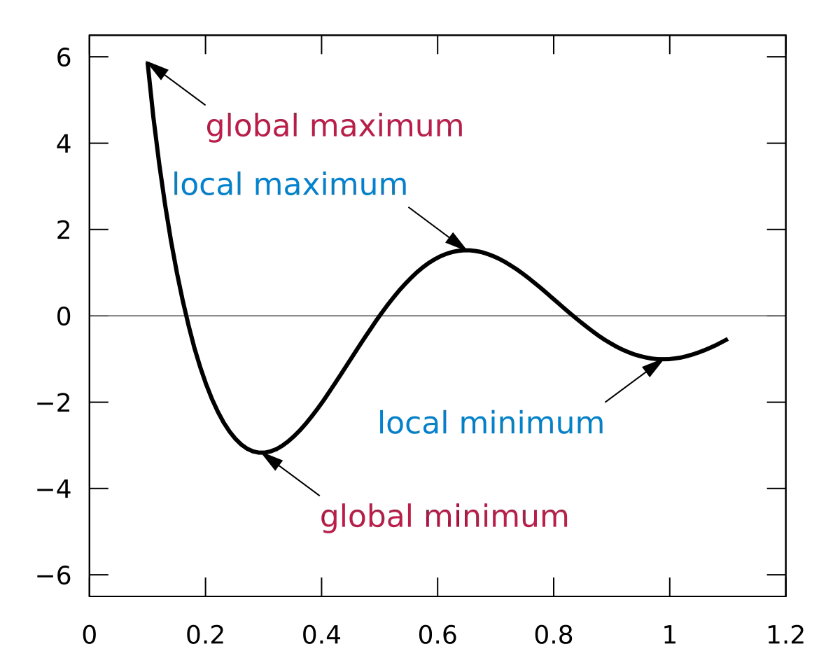
To find the global maxima while using Genetic Algorithm we need to include negative (‘-ve’) sign while evaluating the function, plotting the 3D model using the function values and also in optimum value while plotting in ‘plot3’ command.

f(x,y) = - (f1x*f2x*f1y*f2y)

How a Genetic Algorithm works?

The genetic algorithm works as follows:

1. The algorithm commences by creating a random initial population.
2. It then creates a sequence of new populations. At each successive steps, the algorithm uses the individual member in the current generation to create a new population. To do this, the algorithm performs the following steps:
1. Scores each member of the current population by computing its fitness value. These values are called the raw fitness scores.
2. Scales the raw fitness scores to convert them into a more usable range of values. These scaled values are called expectation values.
3. Selects members, called parents, based on their expectation.
4. Some of the individuals in the current population that have lower fitness are chosen as elite. These elite individuals are passed to the next population.
5. Produces children from the parents. Children are produced either by making random changes to a single parent—mutation—or by combining the vector entries of a pair of parents—crossover.
6. Replaces the current population with the children to form the next generation.
3. The algorithm stops when one of the stopping criteria (which is defined for the condition to stop) is met.

Syntax explaination:

‘ga’ Syntax in MATLAB

In MATLAB ‘ga’ is use to find the minimum of a function using genetic algorithm. Following syntaxes are used to find ‘ga’ in MATLAB.

1. x = ga(fun,nvars) [This finds a local unconstrained minimum, x, to the objective function, fun. nvars is the dimension (number of design variables) of fun.]
2. x = ga(fun,nvars,A,b) [ This finds a local minimum x to fun, subject to the linear inequalities A*x ≤ b. ga evaluates the matrix product A*x as if x is transposed (A*x').]
3. x = ga(fun,nvars,A,b,Aeq,beq) [ This finds a local minimum x to fun, subject to the linear equalities Aeq*x = beq and A*x ≤ b. (Set A=[] and b=[] if no linear inequalities exist.) ga evaluates the matrix product Aeq*x as if x is transposed (Aeq*x').]
4. x = ga(fun,nvars,A,b,Aeq,beq,lb,ub) [ This defines a set of lower and upper bounds on the design variables, x, so that a solution is found in the range lb ≤ x ≤ ub. (Set Aeq=[] and beq=[] if no linear equalities exist.)]
5. x = ga(fun,nvars,A,b,Aeq,beq,lb,ub,nonlcon) [ This subjects the minimization to the constraints defined in nonlcon. The function nonlcon accepts x and returns vectors C and Ceq, representing the nonlinear inequalities and equalities respectively. ga minimizes the fun such that C(x) ≤ 0 and Ceq(x) = 0. (Set lb=[ ] and ub=[ ] if no bounds exist.)]
6. x = ga(fun,nvars,A,b,Aeq,beq,lb,ub,nonlcon,options) [ This subjects the minimization to the constraints defined in nonlcon. The function nonlcon accepts x and returns vectors C and Ceq, representing the nonlinear inequalities and equalities respectively. ga minimizes the fun such that C(x) ≤ 0 and Ceq(x) = 0. (Set lb=[ ] and ub=[ ] if no bounds exist.)]
7. x = ga(fun,nvars,A,b,[],[],lb,ub,nonlcon,IntCon) or x = ga(fun,nvars,A,b,[],[],lb,ub,nonlcon,IntCon,options [ This requires that the variables listed in IntCon take integer values.]
8. x = ga(problem) [ This finds the minimum for problem, where problem is a structure.]
9. [x,fval] = ga(___) [ for any previous input arguments, also returns fval, the value of the fitness function at x.]
10. [x,fval,exitflag,output] = ga(___) [ This also returns exitflag, an integer identifying the reason the algorithm terminated, and output, a structure that contains output from each generation and other information about the performance of the algorithm.
11. [x,fval,exitflag,output,population,scores] = ga(___) [ This also returns a matrix population, whose rows are the final population, and a vector scores, the scores of the final population.]

[In MATLAB Code the ga Syntax which i have used, is explained in comments.]

INPUT ARGUMENTS:-

1. fun – Objective function (Given by function handle or by function name)
2. nvars – Number of Variables (Given by positive integer)
3. A – Linear inequality constraints (Given by real matrix)
4. b – Linear inequality constraints (Given by real matrix)
5. Aeq – Linear equality constraints (Given by real matrix)
6. beq – Linear equality constraints (Given by real matrix)
7. lb – Lower Bounds (Real vector or array)
8. ub – Upper Bounds (Real vector or array)
9. nonlcon – Nonlinear Constraints (function handle or function name)
10. options – Optimization options
11. IntCon – Integer variables (Vector of positive integers)
12. problem – Problem description(structure)

OUTPUT ARGUMENTS:-

1. x – Solution(real vector)
2. fval – Objective function value at solution(real number)
3. exitflag – Reason ga stopped (integer)
4. output – Information about the optimization process(structure)
5. population – Final population(matrix)
6. scores – Final scores(column vector)

Matlab code:

Stalagmite Function Program:

function [F] = stalagmite(input_vector)
x = input_vector(1);
y = input_vector(2);
f1 = (sin(5.1*pi*x+0.5)).^6;
f2 = (sin(5.1*pi*y+0.5)).^6;
f3 = exp(-4*log(2)*((x-0.0667).^2)/0.64);
f4 = exp(-4*log(2)*((y-0.0667).^2)/0.64);
F = -(f1*f2*f3*f4);
end

Main Program:

clear all
close all
clc

% Input to the (Search Space)
x = linspace(0,0.6,100);
y = linspace(0,0.6,100);

% Creating a meshgrid to generate 100x100 matrix
[xx yy] = meshgrid(x,y);

% number of iterations for the GA to run
iteration = 50;

% Evaluating the stalagmite function
for i = 1:length(xx)
    for j = 1:length(yy)
        input_vector(1) = xx(i,j);
        input_vector(2) = yy(i,j);
        f(i,j) = stalagmite(input_vector);
    end
end

figure(1) 
% Generate stalagmite function as a surfc plot
surfc(xx,yy,-f)
colorbar
shading interp % Used to Generate more smoother plot

% Title and Label
xlabel('X-value')
ylabel('Y-value')
zlabel('Function Value')  
title('Stalagmite Function')

% Study 1 :- Unbounded Statistical Behavior
tic
for i = 1:iteration
% Passing 'ga' function
% Here syntax use for 'ga' is [x,fval] = ga(fun,nvars)
% Where 'fun' is objective function (stalagmite function is use as an objective function)
% nvars is number of variable. fval is value of fitness function at x.    
[inputs fval(i)] = ga(@stalagmite,2); 
%50 times 50 values will be stored in fval making it a 1x50 vector, these values are calculated by GA. 
%For each itteration 'i' the output will be printed in 'fval' and the 2 points for that o/p will be printed in the 'inputs' (2x50)
xout(i) = inputs(1);
yout(i) = inputs(2);
end
study_time_1 = toc

figure(2)
% Use subplot function to generate multiple figure in same window
subplot(2,1,1) 
hold on
surfc(xx,yy,-f)  % Generate surfc plot 
shading interp    % Generate more smoother plot

% By using plot3 we can plots multiple sets of coordinates on the same set of axes
plot3(xout,yout,-fval,'marker','o','markersize',5,'markerfacecolor','r')
% labelling and title
xlabel('x-value')
ylabel('y-value')
zlabel('Function value')
title('Unbounded Statistical Behvaiour')

% Second subplot
subplot(2,1,2)
% Plot optimum value
plot(-fval,'linewidth',1.5)  
xlabel('Iterations')
ylabel('Function Maximum')

% Study 2 :- Statistical behavior with Upper and Lower Bounds
tic
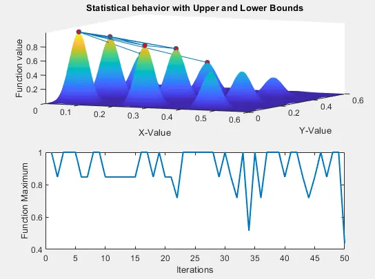
for i = 1:iteration
    % Passing 'ga' function
    % Here syntax use for 'ga' is      [x,fval] = ga(fun,nvars,A,b,[],[],lb,ub)
    % This defines a set of lower and upper bounds on the design variables, x, so that a solution is found in the range lb < x < ub.
    % Where 'fun' is objective function(stalagmite function is used as an objective function)
    % nvars is number of variables. 'fval2' is value of fitness function at x which is 'inputs2'.
    % lb is lower bound and ub is upper bound
    [inputs2, fval2(i)] = ga(@stalagmite,2,[],[],[],[],[0 0],[1 1]);
    xout2(i) = inputs2(1);
    yout2(i) = inputs2(2);
end
study_time_2 = toc;

figure(3)
% Use subplot function to generate multiple figure in same window
subplot(2,1,1)
hold on
surfc(xx,yy,-f) % Generate surfc plot 
shading interp % to generate a more smoother plot

% By using plot3 we can plots multiple sets of coordinates on the same set of axes
plot3(xout2,yout2,-fval2,'marker','o','markersize',5,'markerfacecolor','r')

% labelling and title
xlabel('X-Value')
ylabel('Y-Value')
zlabel('Function value')
title('Statistical behavior with Upper and Lower Bounds')

% Second subplot
subplot(2,1,2)
% Plot optimum value
plot(-fval2,'linewidth',1.5)
xlabel('Iterations')
ylabel('Function Maximum')


% Study 3 :- Increasing Population size for Statistical behavior calculations
% By using optimoptions we create options to optimize 'ga'.
options = optimoptions('ga','populationsize',200);

tic
for i = 1:iteration
    % Passing 'ga' function
    % Here syntax use for 'ga' is [x,fval] = ga(fun,nvars,A,b,[],[],lb,ub,nonlcon,IntCon,options)
    % This defines a set of lower and upper bounds on the design variables, x, so that a solution is found in the range lb ? x ? ub.
    % This Syntax minimize with the default optimization parameters replaced by the values in options.
    % Where fun is objective function(Here stalagmite function is use as objective function)
    % nvars is number of variable. fval is value of fitness function at x.
    % lb is lower bound and ub is upper bound
    [inputs3, fval3(i)] = ga(@stalagmite,2,[],[],[],[],[0 0],[1 1],[],[],options);
    xout3(i) = inputs3(1); % give optimum value to x
    yout3(i) = inputs3(2); % give optimum value to y

end
study_time_3 = toc

figure(4)
% Use subplot function to generate multiple figure in same window
subplot(2,1,1)
hold on
surfc(xx,yy,-f); % Generate surface plot 
shading interp;  % Generate more smoother plot

% By using plot3 we can plots multiple sets of coordinates on the same set of axes
plot3(xout3,yout3,-fval3,'marker','o','markersize',5,'markerfacecolor','r');
% labelling and title
xlabel('X-value')
ylabel('Y-value')
zlabel('Function value')
title('Bounded Statistical Behvaiour With Modified Population Size')

% Second subplot
subplot(2,1,2)
% Plot optimum value
plot(-fval3,'linewidth',1.5)  
xlabel('Iterations')
ylabel('Function Maximum')

clc

% Consolidated Results
fprintf ('\n Study 1 :- Unbounded Statistical Behavior')
fprintf ('\n The Time taken for the study 1 is : %f ',study_time_1)
fprintf ('\n The Co-ordinates of x and y for the Global Maxima of the Function is : %f,%f',inputs(1),inputs(2))
fprintf ('\n The Global Maxima of the Function is : %f',-(stalagmite(inputs)))  

fprintf ('\n \n Study 2 :- Statistical behavior with Upper and Lower Bounds')
fprintf ('\n The Time taken for the study 2 is : %f',study_time_1)
fprintf ('\n The Co-ordinates of x and y for the Global Maxima of the Function is : %f,%f',inputs2(1),inputs2(2))
fprintf ('\n The Global Maxima of the Function is : %f',-(stalagmite(inputs2)))

fprintf ('\n \n Study 3 :- Increasing Population size for Statistical behavior calculation ')
fprintf ('\n The Time taken for the study 3 is : %f',study_time_1)
fprintf ('\n The Co-ordinates of x and y for the Global Maxima of the Function is : %f,%f',inputs3(1),inputs3(2))
fprintf ('\n The Global Maxima of the Function is : %f',-(stalagmite(inputs3)))

Code Explaination

1) We start the program with the usual clear all, close all and clc commands to clear/wipe out all the previous data that was written in the workspace and the compiler window. After this, we commence our optimisation process by inputing the search space to where the global maxima and local maxima are to be found and plotted. With the help of linspace command we feed these values to the x and y. These are column vectors with a matrix size of 1x100 each.

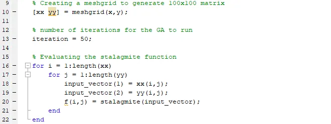
2) Once we have the x and y variables created with the values having equal distances btw them which we had acheived previously with the help of the linspace command, we do the meshgrid to get a 100x100 matrix for x and y. We name these variables as xx and yy and each constituting 100x100 size. Once we do this, we evaluate the stalgamite function by feeding it an input using the input vector which consists of 2 variables x and y. So for each variable pair x and y an output is generated and is stored in the 'f'. We run this loop for 100 times as the length of xx and yy says the same. We conclude the for loop with the use of end commands. Note - we have made use of 2 for loops here to start marching each and every column of each row. So the process starts from the 1st row and goes till the 100th column and then jumps to the 2nd row and goes till the 100 th column of the second row. So this process goes on inside the loop until we achieve the 100th row and 100th column.

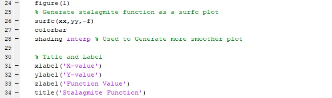
3) After we have the stalgamite values for every pair of x and y run for 100 iterations. We need to start plotting to get a glimpse of how our stalgamite function looks. We initiate the process of plotting with figure command. Once the figure window has been opened we start plotting the surface using, 'surfc' command. Inside the surfc we give inputs for x and y as 'xx' and 'yy'. For the z-axis we need to keep in mind that we are plotting the result of the stalgamite function where we had fed the answers of these calculations done by the stalgamite function in the 'f' variable as executed above with the help of loops and a secondary function (stalgamite function). The 'f' are the results of the function and note that stalgamite function formulas are to calculate the minimum of the members that we had given input through input_vector. These have to be converted to a maximum of the same. This can be achieved by adding a '-' symbol, predecessor to 'f' making all the solutions positive and resulting in a upward trend stalgamite plots. Color bar is used to signify the values of the solution in terms of colors. Referring to, which color signifies what value. So the user, looking at the color can figure out whats the rough value of 'f' at any given point in the plot.

Shading interp gives a smooth plot resulting in a better color accuracy. Once we are done with plotting we do the labelling and titling as per the inputs we have given and the outputs we have obtained.

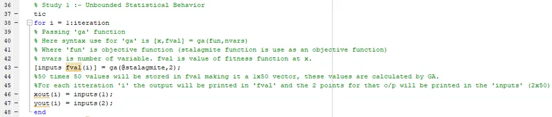
4) So let us do some alterations to this stalgamite and get a better output using the Genetic Algorithm. So to do this, we have to start a for loop. So iteration has been assigned a value of 50 so that the for loop runs for 50 times. The GA has several syntaxes, but we are here going to commence the optimisation using GA with a simple syntax first and march our way upwards to a better optimisation with the help of different syntaxes in GA. The basic GA syntax is [input,fval(i)]=ga(@stalagmite_function,2); is used to perform GA which returns the point of optimum value which is stored in "input" array and the optimum value is stored in "fval" array. Thus every time the iteration takes place, GA is performed and the points and values are stored in separate variables which can be used to plot graph and visualize what is happening in a later session.Two different columns in the input variables are stored in xout and yout arrays. These are basicaly the x and y co ordinate values for which the GA performs its function to get the required output. We end the loop using an 'end' command.

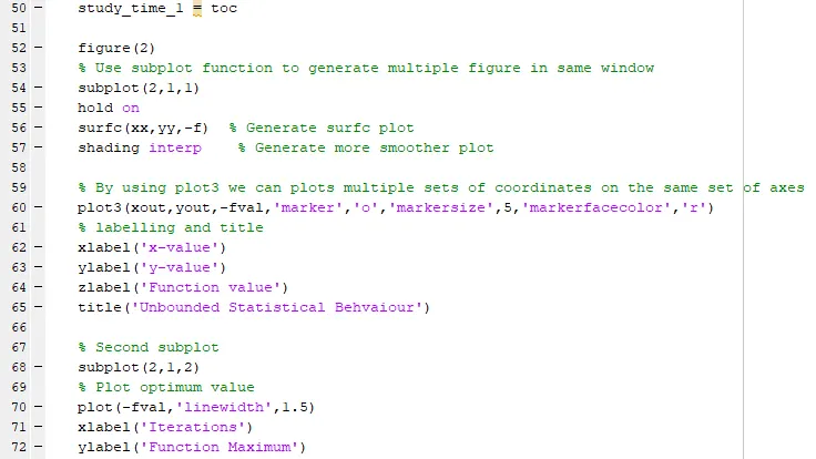
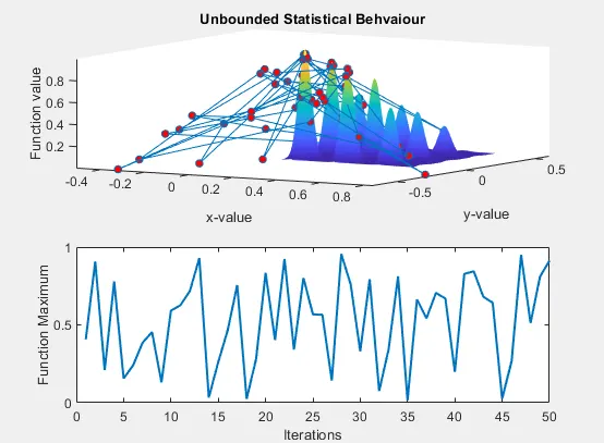
5) The figure 2 has to be created to plot our Case Study 1. The results what we have received through fval,xout and yout will help us plot the upgraded surface plot which will now show a bit more accurate result than the previous one. We make use of the subplot command to open 2 plots in a single figure window. the subplot synatx (2,1,1) means --> Open a 2x1 figure window where i want to plot 2 plots in 2 different rows and 1 column and the last indice '1' means this is going to be my 1st plot. So with the help of 'hold on' we will keep this commands common to all code that will be executed from here.

Under the first subplot we plot the stalagmite function using surfc and 'shading interp' is used to make the plot more smoother along with stalagmite function, the xopt and yopt array is also plotted. In the second subplot, the optimum value function 'fval' is plotted which can be used to see how optimum value changes with different iteration. as we know the genetic algorithm gives only the minimum value we use (-fval) during plot command. We make use of markers to show what are the points the GA has achieved and we have plotted with the stalgamite surface plot.

Inorder to study the behaviour of GA , at first a timer is started to detect the time for the set of code to run, the code calculates the optimum value and the point at which optimum value occurs. The for loops starts with 1 and runs till the size of "iteration" variable which is set to 50 in this case. Every time when the iteration take place, An Optimum value is found using GA whose syntax expects a "function" and the total number of variables used in the function. We use the plot3 command to plot the stalgamite function with the GA enabled, also to depict the number of points in xout and yout in the same plot. After the successful plotting, we label and title the plots as per our inputs and outputs.

A second subplot is created in the similiar manner, the indice 2 here indicates that this is going to be the second sub plot in that same figure window. To just get a rough idea how much our fval is fluctuating over the iterations we get to know the level of optimisation that has been achieved using this GA syntax.

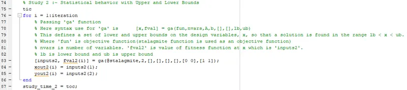
6) Now we jump on to the case study 2, where we start the for loop in the similiar fashion as we did above The [input,fval(i)]=ga(@stalagmite_function,2,[],[],[],[],[0;0],[1;1]); is used to perform GA which returns the point of optimum value which is stored in "input" array and the optimum value is stored in "fval2" array. Thus every time the iteration takes place,GA is performed and the points and values are stored in separate variables which can be used to plot graph and visualize what is happening.Here the boundary conditions are well defined hence we might get reduced random optimum value as compared to case 1.Two different columns in the input variables are stored in xout1 and yout1 arrays.

x = ga(fun,nvars,A,b,Aeq,beq,lb,ub) [ This defines a set of lower and upper bounds on the design variables, x, so that a solution is found in the range lb ≤ x ≤ ub. (Set Aeq=[] and beq=[] if no linear equalities exist.)]

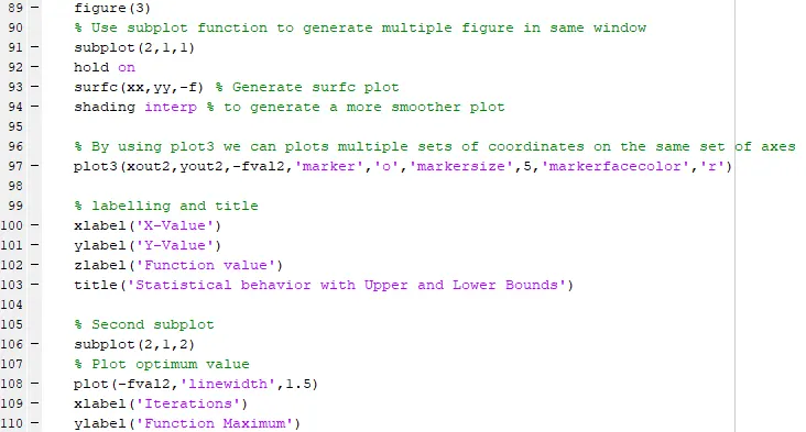
7) Using the 'figure' command, we create a separate window to plot the graph and to visualize the process. The 'subplot' is used to make space for different plot under a single window.

Under the first subplot we plot the stalagmite function using surfc and 'shading interp' is used to make the plot more smoother along with stalagmite function, the xout2 and yout2 array is also plotted. In the second subplot, the optimum value function 'fval2' is plotted which can be used to see how optimum value changes with different iteration. as we know the genetic algorithm gives only the minimum value we use (-fval2) during plot command. The labeling and titling is done for these plots.

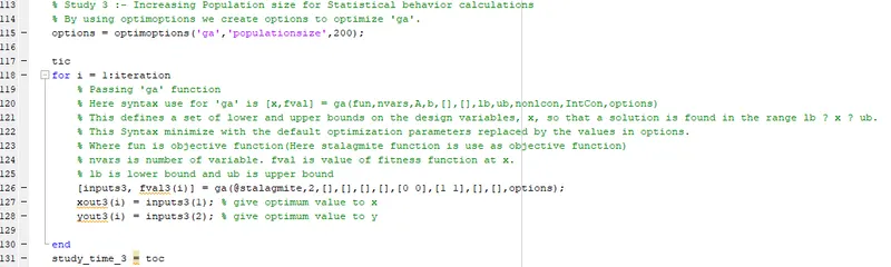
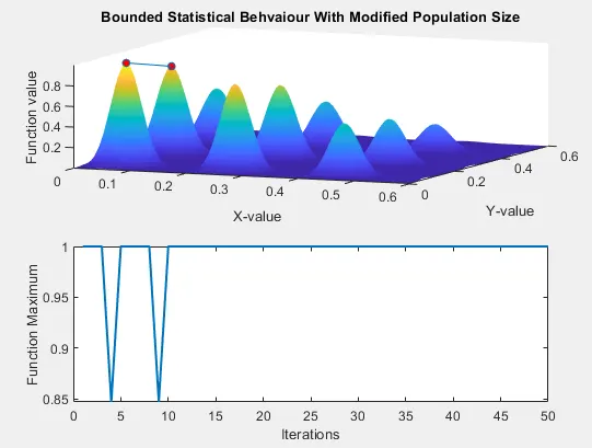
8) The below two lines is used to change the population of the random selection by increasing it by 200. We do this using a special functionc alled optimotions. This is available in the 'doc ga' of the matlab. This function helps us to maintain the population size of 200. This options variable will be fed to the GA function syntax and as an input.

Inorder to study the behaviour of GA , at first a timer is started to detect the time for the set of code to run, the code calculates the optimum value and the point at which optimum value occurs. The for loops starts with 1 and runs till the size of "num_case" variable which is set to 50 in this case. Every time when the iteration take place, A Optimum value is found using GA whose syntax expects a "function" and the total number of variables used in the function.

[input, fval(i)]=ga(@stalagmite_function,2,[],[],[],[],[0;0],[1;1],[],[],options);is used to perform optimum value is stored in "fval" array. Thus every time the iteration takes place,GA is performed and the points and values are stored in separate variables which can be used to plot graph and visualize what is happening.but however along with the boundary conditions mentioned , the population of the random selection is also increased, this allows us to predict the optimum value with the higher precision.Two different columns in the input variables are stored in xopt and yopt arrays.

x = ga(fun,nvars,A,b,[],[],lb,ub,nonlcon,IntCon) or x = ga(fun,nvars,A,b,[],[],lb,ub,nonlcon,IntCon,options [ This requires that the variables listed in IntCon take integer values.] we leave these empty using [].

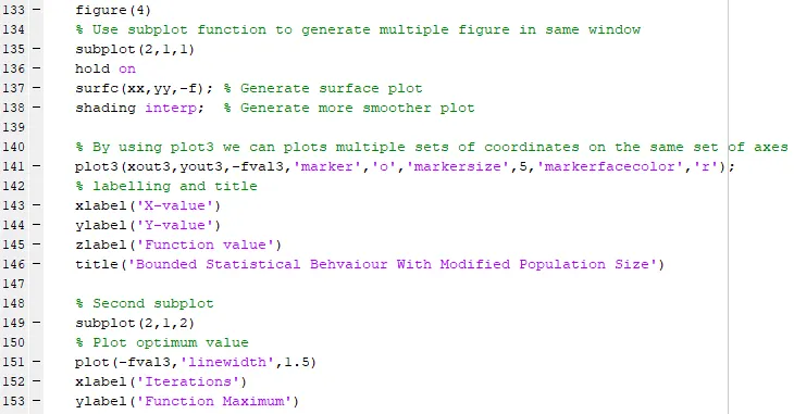
9) Using the 'figure' command, we create a separate window to plot the graph and to visualize the process. The 'subplot' is used to make space for different plot under a single window.

Under the first subplot we plot the stalagmite function using surfc and 'shading interp' is used to make the plot more smoother along with stalagmite function, the xout3 and yout3 array is also plotted. In the second subplot, the optimum value function 'fval3' is plotted which can be used to see how optimum value changes with different iteration. as we know the genetic algorithm gives only the minimum value we use (-fval3) during plot command. The labeling and titling is done for these plots.

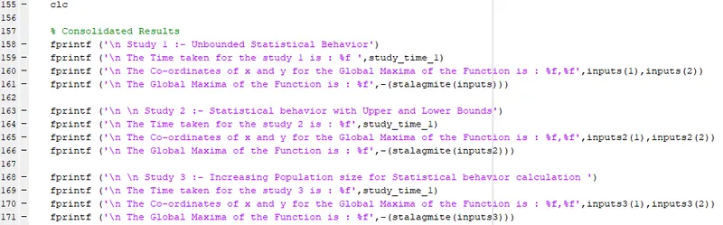
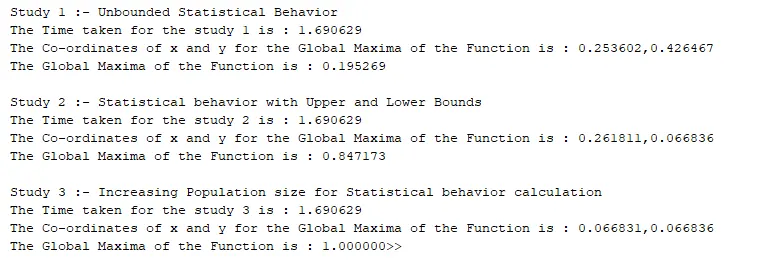
10) Finally, when we are done with all the plotting and labelling. I have takeb a separte list of print statements which is easily readily available for the user to know the answers from these plots. These were achievable using the fprintf commands. The global maxima is achieved when we input the 'inputs' variables to the stalgamite function with the help of -ve sign we get the global maximum value.

Errors faced and rectified during the challenge:

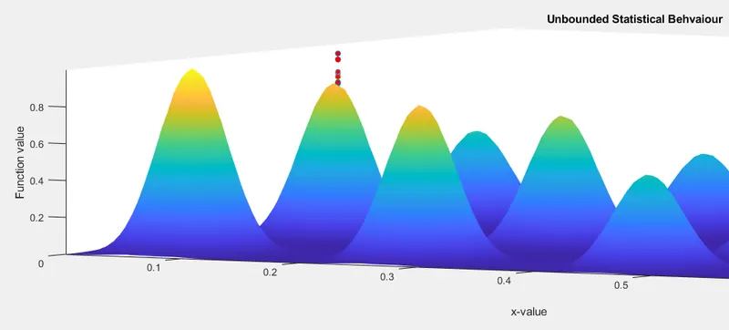
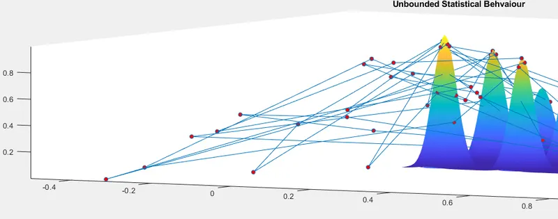
1) Errors faced: I did not achieve the plotting of the xout and yout points for all 50 iterations.

Rectified: because i forgot to use the xout(i) and yout(i). After using the iteration variable with parenthesis i achieved the desired output.

BEFORE AFTER

Output:

Stalgamite function:

CASE - 1:

CASE - 2:

CASE - 3:

Consolidated results:

References:-

1. https://in.mathworks.com/help/gads/ga.html
2. https://www.researchgate.net/profile/Mohamed_Mourad_Lafifi/post/How_can_we_use_Genetic_Algorithm_in_Matlab_such_that_it_returns_same_answer_every_time_we_run_it/attachment/5aa19b874cde266d589024da/AS%3A602004858626049%401520540551775/download/An+Introduction+to+Genetic+Algorithms+Carrjk.pdf
3. https://in.mathworks.com/help/gads/some-genetic-algorithm-terminology.html
4. https://in.mathworks.com/help/gads/how-the-genetic-algorithm-works.html
5. https://towardsdatascience.com/introduction-to-genetic-algorithms-including-example-code-e396e98d8bf3?gi=4b3f2cf1bdf4
6. https://in.mathworks.com/help/gads/what-is-the-genetic-algorithm.html