MATLAB program to plot the PV diagram

A MATLAB program to plot the PV diagram of an OTTO CYCLE for an IC engine application.

Aim:

• A code to create a PV diagram
• To get the output - thermal efficiency of an IC engine.

Theory:

An Otto cycle depicts the working of a petrol or gasoline engine. It comprises of 4 processes - Intake, Compression, Expansion, Combustion. It basically describes the mass of fluid subjected to change in temperature, pressure and volume to show how these entities change when heat is added, stored and removed. The working of an otto cycle (PV Diagram) is show in the figure.

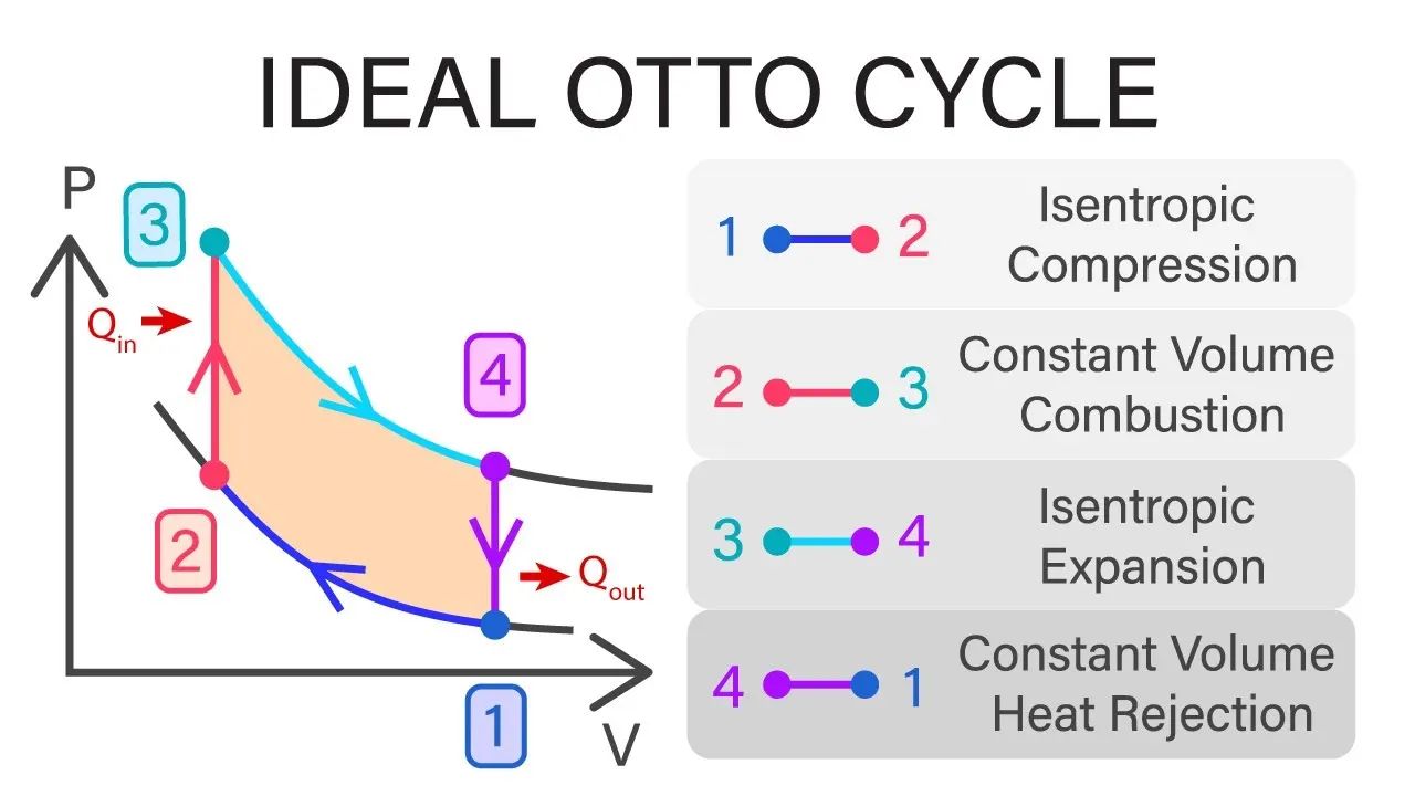
The four-stroke Otto cycle is made up of the following four internally reversible processes: 1–2, isentropic compression; 2–3, constant-volume heat addition; 3–4, isentropic expansion; and 4–1, constant-volume heat rejection.

Formulas:

1) Ideal Gas constant : `PV^gamma =` constant

2) Swept Volume : `Vs = pi/4 * (BORE)^2 * (Stroke)`

3) Clearance Volume :`Vc = (Vs)/(Cr -1`

4) Compression/Expansion Volume : `V=(1+0.5(Cr−1)[R+1−cosθ−(R^2−sin^2 θ)^0.5])⋅Vc`

5) Ideal Gas Constant : `P*V*T =` Constant

6) Efficiency : `eta = [1 - (T1)/(T2)] * 100`

P = pressure (Pa)

V = volume `(m^3)`

T = temperature(K)

Cr = compression ratio

Vs = Swept volume

Vc = Clearance volume

a = Crankpin radius = (`(stroke)/2`)

η = thermal efficiency (%)

Program to calculate the Engine Kinematic:

The Function Program:

function [V] = engine_kinematic(bore,stroke,cond_rod,Cr,start_angle,end_angle)
% Inputs
%bore = 0.1;
%stroke = 0.1;
%cond_rod = 0.15;
%Cr = 12;

%Calculation of Volumes
V_swept = pi/4 * (bore)^2 * stroke;
V_clear = V_swept / (Cr-1);

% for variable angles
theta = linspace(start_angle,end_angle,100);
%theta = linspace(0,720,720);

%% Variation in volume 'V' inside the combustion chamber as crank angle changes
a = stroke / 2;
R = cond_rod / a;
term_1 = 0.5 * (Cr - 1);
term_2 = R + 1 - cosd(theta);
term_3 = (R^2 - sind(theta).^2).^0.5;
V = ( 1 + term_1 * (term_2 - term_3)).* V_clear;
plot(theta,V)

end

Program to plot the PV Diagram of an Otto Cycle:

%Program to solve an Otto cycle using MATLAB
clear all
close all
clc

%Engine geometric parameters
bore = 0.1;
stroke = 0.1;
cond_rod = 0.15;
Cr = 12; %Compression ratio = Cr

%Swept volume and clearance volume
V_swept = pi/4 * (bore)^2 * stroke;
V_clear = V_swept / (Cr-1);

%state variables at state point 1 
p1 = 101325;
t1 = 500;
gamma = 1.4;
v1 = V_swept + V_clear;
v2 = V_clear;

%state variable at state point 2
    % For an isentropic process, pv^gamma=constant
    % p1v1^gamma=p2v2^gamma; %p2=p1*(v1/v2)^gamma = p1*r_c^gamma
p2 = p1 * Cr^gamma;
    %To compute t2, we will use the ideal gas equation pv/t =constant
    %p1v1/t1=p2v2/t2 ; t2= p2*v2*t1/(p1*v1)
t2 = (p2*v2*t1) / (p1 * v1);

constant_c = p1 * v1^(gamma);
V_compression = engine_kinematic(bore,stroke,cond_rod,Cr,180,0);
P_compression = constant_c ./ V_compression.^gamma;

%state variable at state point 3
v3 = v2;
t3 = 2300;
    % p3*v3/t3=p2*v2/t2 ; p3=p2*t3/t2 (v2 cancels out)
p3 = p2*t3/t2;

constant_c = p3 * v3^(gamma);
V_expansion = engine_kinematic(bore,stroke,cond_rod,Cr,0,180);
P_expansion = constant_c ./ V_expansion.^gamma;

%state variables at state point 4 
 v4=v1;
    %p3v3^gamma=p4v4^gamma ; p4=p3*(v3/v4)^gamma
p4=p3*(v3/v4)^gamma; 
    %p3*v3/t3=p4*v4/t4
t4=(p4*v4*t3)/(p3*v3);

%Efficiency
eff_otto=(1-(t4-t1)/(t3-t2))*100;

%Plotting the Otto Cycle
figure(2);
xlabel('Volume in m^3')
ylabel('Pressure in Pa')
title('PV Diagram of an Otto Cycle')
axis([0e-4 0.00089 0 6e6])
hold on
plot(v1,p1,'*','color','r');
plot(V_compression, P_compression,'color','b');
plot(v2,p2,'*','color','r');
plot(v3,p3,'*','color','r');
plot(V_expansion, P_expansion,'color','b');
plot(v4,p4,'*','color','r');
plot([v1 v4],[p1 p4])
plot([v2 v3],[p2 p3])
text(v1,p1,'1','FontSize',6)
text(v2,p2,'2','FontSize',6)
text(v3,p3,'3','FontSize',6)
text(v4,p4,'4','FontSize',6)

Programming explaination:

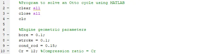
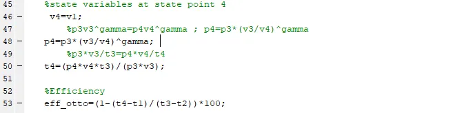
1) The standard first 3 lines of code to clear and close all the previous data including the workspace in matlab. Whenever we begin solving a problem, it is very important for us to assign the initial quantities such as bore, stroke, connecting rod length and compression ratio.

2) After defining the initial quantities of the engine parameters. Let us straight away jump to calculate the Swept Volume and Clearance Volume. Swept volume is the volume btw BDC and TDC positions of a piston. The clearance volume is the volume is the volume that remains in the cylinder when piston is at the TDC position.

3) So in the PV diagram we can see that our origin is point 1 or state point 1. So calcualting, Volumes at point 1 (v1) is the sum of clearance and swept volumes. Volume at point 2 (v2) is the clearance volume. With the calculations of V1 and V2, I have also mentioned the values of P1 = 1 atm = 101325 Pa, T1 = 500K and `gamma`= 1.40

4) At state point 2, we calculate the remaining variables using the following equations:-

Now for a reversible adiabatic process we know that, `P* V^gamma = constant` `-> (A)`

Therefore we can say that; `p1 * v1^ (gamma) = p2*v2^(gamma)`

In the process 1-2 wehn a fixed amount of fuel-air mixture enter the combustion chamber, the variables like pressure, volume and temperature will change.

So we can say that `(p*v)/(t) = c` `-> (B)`

`((p1*v1)/(t1)) = ((p2*v2)/(t2))`

`t2 = (p2*v2*t1) / (p1 * v1)`

Hence we have calculated t2 here.

5) After the state point 2, We are gonna calculate the constant value using the ideal gas equation.

V_compression =engine_kinematic(bore,stroke,cond_rod,Cr,180,0)

V_compression is one array which stores all the values passed by the function piston_kinematics, where we have written it separately in MATLAB. This process is called as "calling a function" and that is what we have done is line 32.

It is worth to note that this function is altogether a different program which will be used to plot the PV diagram for different input parameters in engine dimensions and crank shaft angle.

While specifying one should understand that during compression piston moves from BDC to TDC so the initial crank angle is going to be 0° to 180° and the final crank angle is going to be 180° to 0°.

The reason why a function was created and called to this code is because we had to find a series of different expansion and compression volume values that we give as an input through linspace in the `theta`.

P_compression is calculated by `P_compression = (constant c)/(Vcompression)^gamma`

6) State variables at point 3 is determined by the following calculations. Since 2-3 is a constant volume process v3 = v2. `p/t = c` is used to determine variables to calculate the values of p3. Here we consider `T_3` as 2300k because we assume that heat is added using an external entity like fuel.

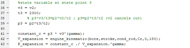
Now coming to the V_expansion, It is similar to the previously calculated compression formula where constant c is calculated first using pressure and volume at point 3 p3 and v3. Further the function is called again in the similiar manner. The values are stored in an array V_expansion and P_expansion.

7) In the state variables at point 4 the values of p4, T4 are determined in the same fashion. Now at point 4; piston is at BDC, therefore, the volume will be the sum of clearance and swept volume (i.e. v1=v4). The variables pressure and temperature can be determined using equations A and B respectively, as mentioned above.

Finally, we have to calculate the thermal efficiency of the Otto Cycle.

Calculating the thermal efficiency for the Otto cycle. `eta_(th) =` work done`/`heat supplied

Work done = Heat Supplied - eat rejected. (Heat is supplied from process 2 to 3 and Heat is rejected from process 3 to 4.)

On simplifying;

`eta_(th) = ((t3-t2) - (t4-t1))/(t3 - t2)`

`eta_(th) = 1 - ((t4-t1)/(t3-t2))`

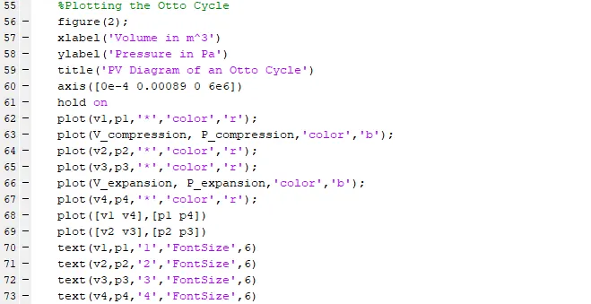
8) Plotting of the points for Pressure v/s Volume is done using the plot command.

plot(v1,p1,'*','color','b') - The '*' is used as a marker for volume and pressure that are indicated for state variable values at point 1,2,3 and 4.

plot(V_compression, P_compression,'color','b') and plot(V_expansion, P_expansion,'color','b') gives us a nice curve and depicts that the area under the curve which is actually less and true.

As the assignment also tells us to draw 2 vertical line connecting state points 2,3 and 4,1. we can do this using the plot([v1 v4],[p1 p4])
plot([v2 v3],[p2 p3]) commands.

Text commands were used to indicate the texts for the x,y axis and the title of the graph

Errors faced and rectified during programming:

1) Error: Not using the element wise operate '.' led me to this error.

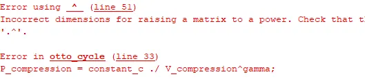
Steps taken to overcome: I used the '.' in the line 33 after V_compression.^gamma. The error was resolved.

2) Error: I was not getting a smoot curve, instead a flat curve was the out put like you can see in the figure plot.

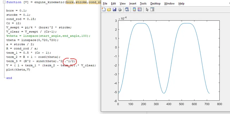
Steps taken to overcome: I mistakenly typed 1/2 thinking matlab will interpret it has 0.5, but then i remembered the precedence of operator concept in MATLAB. The error was corrected when i used 0.5 instead of 1/2.

Output of the Program:

• The PV Diagram plotted generated by the MATLAB code is as follows:

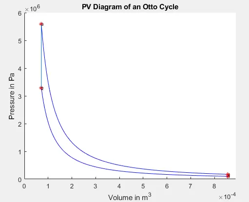
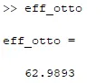
• The Efficiency of the Otto cycle is calcuated and the result is, `eta_(ot t o`= 62.9893%