Week 3 - Solving second order ODEs
Pendulum Oscillation using Second Order Differential Equation
Aim: Creating a program in MATLAB to solve the following ODE and simulating the motion of a simple pendulum using ODE function.
`(d^2(theta))/(dt^2)+b/m(d(theta))/(dt) + g/L sin(theta) = 0`
Objective:
- To create a program and solve the Second ODE
. -
To create a program in MATLAB that will simulate the pendulum motion.
Theory: The equation of motion of a simple pendulum is based on Newtons second law of motion. A simple pendulum consists of a ball (point-mass) m hanging from a (massless) string of length L and fixed at a pivot point P.
The initial conditions for this problems are:
`theta` : the deflection angle
L: Length of pendulum (1m)
m: Mass of pendulum (1kg)
g = acceleration due to gravity (9.81`m/s^2`)
b = damping coefficient (0.1)
Initial angular velocity: 5m/s
When the pendulum is agitated by an angle `theta`. The gravity causes the pendulum to deccelerate acting as a resistance. Thus which decreases the angular velocity and displacement over the time.
If there was no resistance for this motion it would move infinitely, but the point to note here is the surrounding air and gravity, provdes provides resistance to this motion hence damping the motion of the pendulum and finally bringing it to halt.
The damping is calculated using the damping coefficient (b).
`(d(theta))/ dt` : change in`theta`w.r.t. time which can also be said as velocity.
`(d^2(theta))/(dt^2)` : rate of change `theta`w.r.t times square which significates the displacement.
The equation of motion for the pendulum is given as:
`(d^2(theta))/(dt^2)+b/m(d(theta))/(dt) + g/L sin(theta) = 0`
If the amplitude of angular displacement is small, so the small angle approximation holds true and then the equation of motion reduces to the equation of simple harmonic motion. Here our goal is to reduce a second order ODE to 2 singe order ODE, as the degree is 2. To begin this derivation.
Let us assume;
 ..............................................................................(A)

We know that;
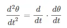
Hence,
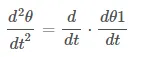
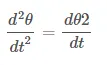
Replacing the values of `(d^2(theta))/(dt^2)`;
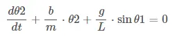
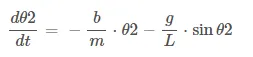 ............................................(B)
Rearranging equation A and B in a matrix form, we can write is as,
 ......................................(C)
Matlab code:
Function Program (ODE_func):
%Function for the pendulum motion to solve the Second ODE
function [dtheta_dt] = pendode_func(time,theta,b,g,L,m)
theta1 = theta(1);                  %Displacement(rad)
theta2 = theta(2);                  %Velocity(rad/s)
dtheta1_dt = theta2;
dtheta2_dt = -(b/m)*theta2-(g/L)*sin(theta1);
dtheta_dt = [dtheta1_dt;dtheta2_dt];
end
Main Program :
close all
clear all
clc

b = 0.5;    %Damping coefficient is(Dimensionless)
g = 9.81;   %Acceleration due to Gravity(m/s^2)
L = 1;      %Length of the string(m)
m = 1;      %Mass of the bob(kg)

% Initial condition; time to start at 0 and angular displacement to start
% from 3.
theta_0 = [0 ; 3];         %[angular displacement, angular velocity]
t_span = linspace(0,20,1000); %Creating 1000 equal spaced timespan array between 0 and 20 sec

%Solving for the ODE
[t results] = ode45(@(t,theta) ode_func(t,theta,b, g,L, m),t_span,theta_0);

%Plotting of Result v/s Time
figure(1)
grid on

%Plotting and figure labelling inputs
plot(t,results(:, 1))
hold on
plot(t,results(:, 2))
xlabel('Time')
ylabel('Angular Velocity and Displacement')
legend('Time','Velocity')
hold off

%Ploting the angular velocity VS position
figure(2)
plot(results(:,1),results(:,2))
xlabel('position')
ylabel('angular velocity')

%Plotting the Pendulum simulation figure for each step of 'i'
figure(3)
hold on
ct = 1;   %Initial Counter Value
for i=1:length(t_span)
   %Hanging position of pendulum
   x0 = 0;
   y0 = 0;

   %Pendulum movement
   y1 = -L*cos(results(i,1));
   x1 = L*sin(results(i,1));
   %Hanging Point
   plot(x0,y0,'s','MarkerFaceColor','b','MarkerSize',10)
   hold on
   axis([-1 1 -1.5 0])  %Defining the axis

   %Hanging line
   plot([-1,1],[0,0],'linewidth',3,'color','c');

   %Pendulum Line
   plot([x0 x1],[y0 y1],'linewidth',3,'color','b');

   %Pendulum Ball
   plot(x1,y1,'o','MarkerFaceColor','r','MarkerSize',30)
   xlabel('Angular Displacement')
   title('Pendulum Simulation')
   plot([x0 x1], [y0 y1], '-bo', 'LineWidth', 3, 'MarkerSize', 20, 'MarkerFaceColor', 'r', 'MarkerEdgeColor', 'r', 'MarkerIndices', 2)
   hold off
   pause(0.03);
   M(ct) = getframe(gcf); %Frame capuring stored in A
   %Create Gif
   fprintf('Creating GIF- Progress... %d\n', ct);
   %M(ct) = getframe()
   filename = 'animation.gif';
   img = frame2im(M);
   [A, map] = rgb2ind(img,256);
   if ct == 1
      imwrite(A,map,filename,'gif','LoopCount',Inf,'DelayTime',0.03);
   else
      imwrite(A,map,filename,'gif','WriteMode','append','DelayTime',0.03);
   end
   %imwrite(img, 'animation.gif', 'DelayTime', .005, 'Compression', 'bzip',
'WriteMode', 'Append')
   %imwrite(A,map,'animation.gif','gif','WriteMode','append','DelayTime',1);
   ct = ct + 1; %Counter incremented for next iteration
end

%Animation of the simulation of a pendulum oscillation
movie(M);
videofile = VideoWriter('Pendulum_simulation.avi'); %Frame stored in A will be stored as video
open(videofile);
writeVideo(videofile,M); %Video is created
close(videofile);
Programming explaination:
1) The standard first 3 lines of code to clear and close all the previous data including the workspace and the Input parameters are defined in the code as mentioned below.
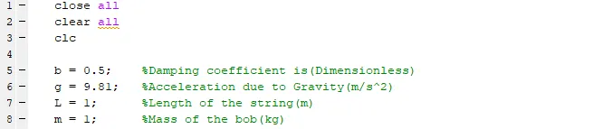
2) The initial quantities are specified and an Input for time span or period over which pendulum oscillates is given.

3) Separate program is written by using ‘function’ in MATLAB to calculate dθ`/dt, where `θ` is the column vector and is given by `θ = [θ1; θ2]. Here θ1 represents angular velocity and θ2 represents angular displacement. After doing so we have values of `(d theta_1)/(dt)`. Now, here comes the heart of our program, where we will first mention that our given equation is a function of 'time' and 'theta' using inbuilt function 'ode45'. It is a solver used to solve and first ODEs. Here we call our function 'ode_func' that will take the initial condition values and return the answer in variable [time,result]. As our equation is a function of time and theta, we will mention 'timespan' and 'theta_0' in the end. What it does is, it has the values needed to be input and time limits needed for calculation in the ode45 solver. This is a variable which we use to showcase out 'time' and 'theta' function. The results hold a 1000x2 matrix where the 1st column consists of the result - angular velocity and the seconf column consists of the result - angular displacement. the variable 't' holds the values of different time interval where results(1000,1) and results(1000,2) was calculated.

4) Once the array of [t ,result] is created and assigned, we will plot graph of 'Displacement v/s Time' and 'Angular Velocity v/s Time'. For 'Displacement v/s Time' we have written plot(t,result(:,1)), which means it will take all the answer from first column and plot versus time. For 'Angular Velocity v/s Time' we have written plot(t,result(:,2)), which means it will take all the answer from second column and plot versus time. Hold on is used to have a complete curve in one frame. And we have named this plot as figure(1). Labelling is done and lastly the hold command is set to 'off'.
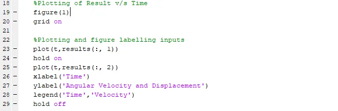
5) Nextly, I have opened a figure(2) to plot a graph btw the pendulum positiona and the angular velocity. I have used the same methods to plot this graph as well. The results variable consists of all the values we are looking for, to plot this graph.

6) We can find the value of the bob at different location of 'theta1' that is our angular velocity. This is why, we will use our 1st column of the result matrix. From above figure. We know that,
r = L;
x = x1;
y = y1;
and the pendulum is hung at an origin (x0,y0) =(0,0).
Here, we will use a for loop for 'i' starting from one to length of our array result storing velocity and displacement values. Basically this, will iterate for 1000 variables.
The hanging position x0,yo does not change. But for x1 and y1, our displacement value will change at every iteration and so will our x1 and y1 position.
The equations are;
%Pendulum movement
y1 = -L*cos(results(i,1));
x1 = L*sin(results(i,1));
- For loop is used from i=1: length(t_span) where t_span is no of times the angular displacement and angular velocity is to be calculated from time t = 0 to 20sec.
- In the program ‘y’ denotes the angular displacement. A new variable Y1 is created to access individual value at each time from array ‘y’.
- x and y coordinate of mass of a pendulum is calculated for each time as x1 and y1
- An Axis function {axis([-1 1 -1.5 0])} is used to show that we can get our actual co-ordinates necessary to plot the figures and ultimately start an animation from the point we desire.
- Line is created from (x0,y0) to (X1,y1) which represents string of a pendulum.
- Bob or mass of a pendulum is created by using a ‘marker’ command with suitable size of marker and colour.
- Tittle is given to the image with a 'title' command.
- 'hold off' command is used to erase images from the privious time step.
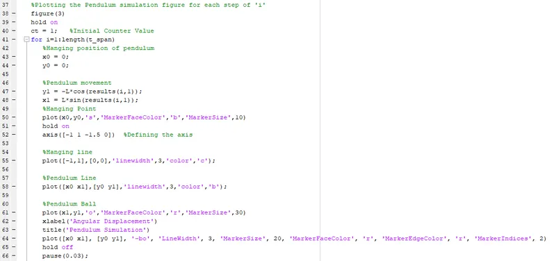
7) M variable stores all the frames that was displayed in each itteration. So ct indicates the count by which the sequence was followed to feed the frame values to the variable M.
Also i made an attempt to use the imwrite command and generate a GIF. Since i have made use of the video writer and movie commands here, i have commented out the program code for GIF generation. Lastly, ending the loop with a ct=ct+1 counter is very important as, we have to jump to the next iteration and this is the only line of code where we tell the for loop to do this job. Always end a function with a 'end'.
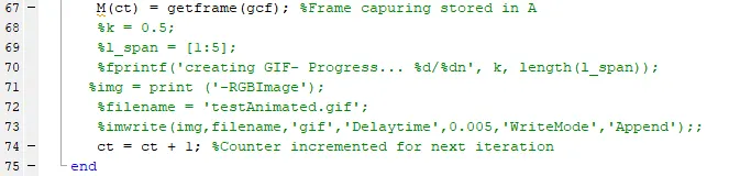
8) Hence, the last part of the program is to create an aniamtion and once all our frames are captured, we will make a video out of it using a movie function. Movie will take the input as frames stored in M. We will make a variable videofile, where we use function VideoWriter. Here, we store the name of video in an 'avi' format in an uncompressed version. Then, we actually start the video creation process using an open function, where the name of the video will be created - 'pendulum_simulation'. Then we use the writeVideo function to create a video of the name ''pendulum_simulation' in uncompressed version with the frames stored in M. Once that is done, we will use close function to close that videofile.

Errors faced and steps took to overcome:
1) Error faced: I did not use the hold off command after plotting of pendulum. This did not remove position of string and ball at prior location.
Steps taken to Overcome: After using the hold off command. I got a clean figure where the previous position of the string and ball did not leave a trace, resulting the desired simulation.
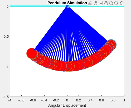
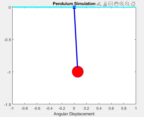
BEFORE AFTER
2) Error faced: I did not use a negative sign before cosine function. Which resulted the pendulum simulation in the wrong quadrant of the plot graph.
Steps taken to Overcome: A negative sign with the cosine in the y1 variable. Solved my problem.
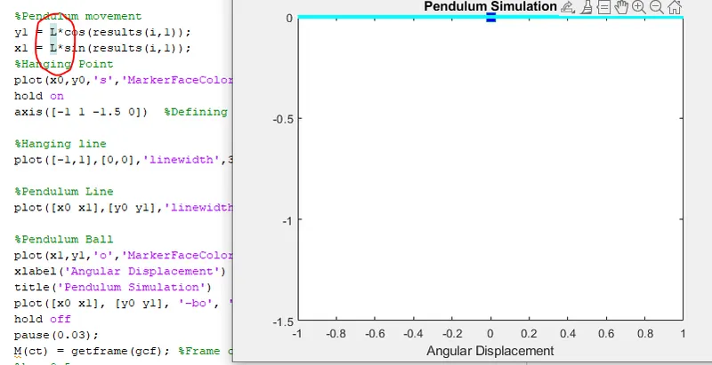
Result:
- For each value in time, an image that represents the position of the pendulum was stitched to an animation creating a video file. This was made possible using the for loop.
- Making use of the ode45 solver to integrate first order ODE and converting the higher order ODE to first order ODE and solving it using ode45 solver.
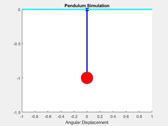
GIF IMAGE
The final animation of the Pendulum oscillation is created and our aim is fulfilled.
The link to the final animation video - https://youtu.be/6oaTG759erk