Curve fitting of the Specific heat and Temperature data using the Polynomial equations in MATLAB

Curve fitting of the Specific heat and Temperature data using the Polynomial equations in MATLAB

Aim:

• Write a code to fit the linear and cubic polynomial for the Cp data.
• To Plot the linear and cubic fit curves along with the raw data points. Title and axes labels are a must, legends could be shown if necessary.
• To Explain the parameters used to measure the fitness characteristics for both the curves.
• To find the methods of improvement of the cubic fit.

Theory:

Curve fitting is the process of constructing a curve, or mathematical functions, which possess the closest proximity to the real series of data. By curve fitting, we can mathematically construct the functional relationship between the observed dataset and parameter values, etc. It is highly effective in the mathematical modeling of some natural processes.

Assume data points (x1,y1) , (x2,y2) , (x3,y3) , ... (xn,yn) and assume the best fit for these set of points will be y = f(x), the criterion under which the equation of the curve will be the best fit possible is as follows,

How to choose the best fit?

Upon finding a curve which satisfies the data points there are 4 quantities which help us measure the goodness of fit criteria or how well the equation is a representing the datapoints. The methods are,

• The sum of squares due to error (SSE)
• R-square
• Adjusted R-square
• Root mean squared error (RMSE)

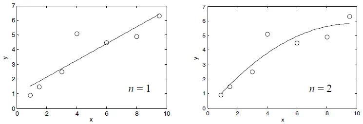
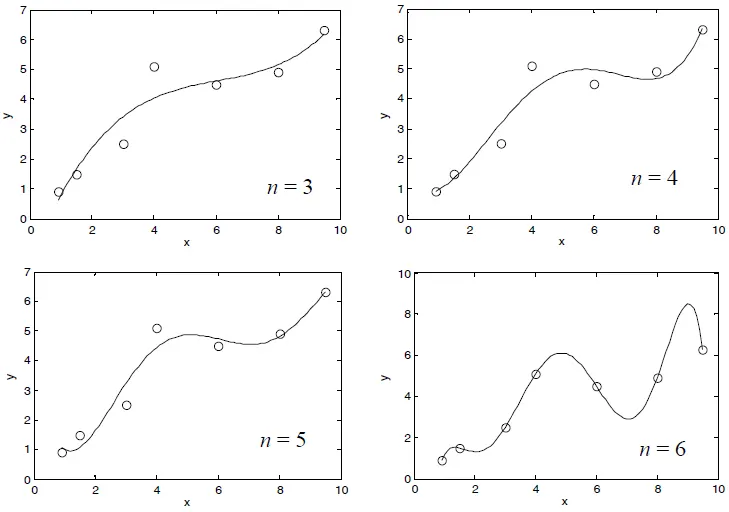
An example for the different types of fit can be seen in the images below considering some random set of seven points: (0.9,0.9),(3,2.5),(4,5.1),(6,4.5),(8,4.9) and (9.5,6.3), The points are fitted using the polyfit function with polynomials of degrees 1 through 6. Each plot in figures shows the same data points, marked with circles, and a curve-fitted line that corresponds to a polynomial of the specified degree.

Programming:

The following matlab program is focussed on a dataset where the variation of the specific heat (`C_p`) with the variation in temperature consists a 3200x2 original data points are predefined in the program. Our aim here is to compare and create different curve fit models that would best fit the original data curve with lowest possible error by trying to maintain the good condition of the polynomial equations

Before jumping straight to using the matlab built-in library functions to carry out the curve fitting process, the same process can be carried out manually by mathemetical computation with various theoretical concepts and strategies. It totally depends on the individual to choose their favourable method in order to get the output

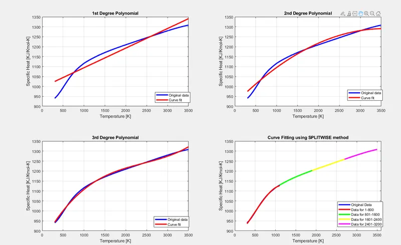
The matlab program explaining the mathematical computation for the 1st, 2nd and 3rd order polynomial curve fits that are - linear, quadratic and cubic curve fit, is explained below within the code snippet and the output plots,

clear all
close all
clc
 
% preparing the data
cp_data = load('data'); %loads the data and then saves it in the form of array
T = cp_data(:,1); % stores first column as temperature
cp = cp_data(:,2); % stores second column as cp

plot(T,cp,'linewidth',3,'color','b')
xlabel('Temperature [K]') % labelling x-axis
ylabel('Specific Heat [KJ/Kmol-K]')  % labelling y-axis
hold on

% curve fit for 1 degree polynomial    
subplot(2,2,1)
figure(1)
coeffs_1 = polyfit(T,cp,1); % calculates the value of coefficients of 1 degree polynomial equation
predicted_cp1 = polyval(coeffs_1,T); % calculates the value of cp based on the value of coefficient and temperature
plot(T,cp,'linewidth',3,'color','b')
xlabel('Temperature [K]') % labelling x-axis
ylabel('Specific Heat [KJ/Kmol-K]')  % labelling y-axis
hold on
plot(T,predicted_cp1,'linewidth',3,'color','r')
xlabel('Temperature [K]') % labelling x-axis
ylabel('Specific Heat [KJ/Kmol-K]')  % labelling y-axis
legend('Original data','Curve fit') % providing legends to differentiate the data
title('1st Degree Polynomial') % giving a title
grid on
hold off


% curve fit for 2 degree polynomial    
subplot(2,2,2)
%figure(2)
coeffs_1 = polyfit(T,cp,2); % calculates the value of coefficients of 2 degree polynomial equation
predicted_cp1 = polyval(coeffs_1,T); % calculates the value of cp based on the value of coefficient and temperature
plot(T,cp,'linewidth',3,'color','b')
xlabel('Temperature [K]') % labelling x-axis
ylabel('Specific Heat [KJ/Kmol-K]')  % labelling y-axis
hold on
plot(T,predicted_cp1,'linewidth',3,'color','r')
xlabel('Temperature [K]') % labelling x-axis
ylabel('Specific Heat [KJ/Kmol-K]')  % labelling y-axis
legend('Original data','Curve fit') % providing legends to differentiate the data
title('2nd Degree Polynomial') % giving a title
grid on
hold off


% curve fit for 3 degree polynomial    
subplot(2,2,3)
%figure(3)
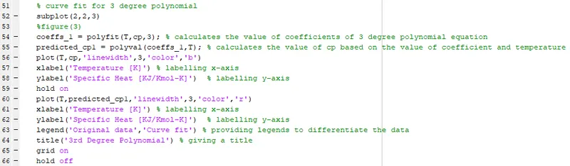
coeffs_1 = polyfit(T,cp,3); % calculates the value of coefficients of 3 degree polynomial equation
predicted_cp1 = polyval(coeffs_1,T); % calculates the value of cp based on the value of coefficient and temperature
plot(T,cp,'linewidth',3,'color','b')
xlabel('Temperature [K]') % labelling x-axis
ylabel('Specific Heat [KJ/Kmol-K]')  % labelling y-axis
hold on
plot(T,predicted_cp1,'linewidth',3,'color','r')
xlabel('Temperature [K]') % labelling x-axis
ylabel('Specific Heat [KJ/Kmol-K]')  % labelling y-axis
legend('Original data','Curve fit') % providing legends to differentiate the data
title('3rd Degree Polynomial') % giving a title
grid on
hold off

% curve fitting - improving the fit by using centering and scaling
temperature1 = T(1:800); % temperature is divided in 1 to 800
predicted_cp1 = cp(1:800);  % cp is divided in 1 to 800
 
temperature2 = T(801:1600); % temperature is divided in 801 to 1600
predicted_cp2 = cp(801:1600);  % cp is divided in 801 to 1600
 
temperature3 = T(1601:2400); % temperature is divided in 1601 to 2400
predicted_cp3 = cp(1601:2400);  % cp is divided in 1601 to 2400
 
temperature4 = T(2401:3200); % temperature is divided in 2401 to 3200
predicted_cp4 = cp(2401:3200);  % cp is divided in 2401 to 3200
 
% curve fit for 1 to 800 using centering and scaling
coeffs1 = polyfit(temperature1,predicted_cp1,3); %  calculates the value of coefficients of 3 degree polynomial equation
cp1 = polyval(coeffs1,temperature1);  % calculates the value of cp1 based on the value of coefficient1 and temperature1
 
% curve fit for 801 to 1600 using centering and scaling
coeffs2 = polyfit(temperature2,predicted_cp2,3);  % calculates the value of coefficients of 3 degree polynomial equation 
cp2 = polyval(coeffs2,temperature2); % calculates the value of cp2 based on the value of coefficient2 and temperature2
 
% curve fit for 1601 to 2400 using centering and scaling
coeffs3 = polyfit(temperature3,predicted_cp3,3);  % calculates the value of coefficients of 3 degree polynomial equation 
cp3 = polyval(coeffs3,temperature3); % calculates the value of cp3 based on the value of coefficient3 and temperature3
 
% curve fit for 2401 to 3200 using centering and scaling
coeffs4 = polyfit(temperature4,predicted_cp4,3);  % calculates the value of coefficients of 3 degree polynomial equation 
cp4 = polyval(coeffs4,temperature4); % calculates the value of cp4 based on the value of coefficient4 and temperature4

% plotting 
subplot(2,2,4)
%figure(4)
plot(T,cp,'linewidth',3,'color','b') % original data
 
hold on
plot(temperature1,cp1,'linewidth',3,'color','r') % data from 1 to 800
plot(temperature2,cp2,'linewidth',3,'color','g') % data from 801 to 1600
plot(temperature3,cp3,'linewidth',3,'color','y') % data from 1601 to 2400
plot(temperature4,cp4,'linewidth',3,'color','m') % data from 2401 to 3200
 
axis([0 3600 900 1350]) % setting the axiz limits
hold off
 
xlabel('Temperature [K]') % labelling x-axis
ylabel('Specific Heat [KJ/Kmol-K]') % labelling y-axis
title('Curve Fitting using SPLITWISE method') % giving a title to the plot
legend('Original Data','Data for 1-800','Data for 801-1600','Data for 1601-2400','Data for 2401-3200') 
grid on

Programming explaination:

1) The standard first 3 lines of code to clear and close all the previous data including the workspace and the Input parameters are defined in the code as mentioned below.

2) To assign 2 variables of the 2 columns of data in the file is loaded using the "load(file_name)" command. We assign this data to a variable cp_data which is a 3200x2 matrix. The cpdata(:,1) signifies the temperature data and the cpdata(:,2) signifies the cp_data. Where these values are assigned to the temperature 'T' variable and specific heat to the 'Cp' variable.

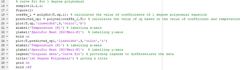
3) The curve fit for 1st degree polynomial is created, “polyfit” command is used to calculate the values of the coefficients of the polynomial equation and then with “polyval”, the values of “predicted_cp1” is calculated with coefficients and the temperature as an input. This step has to be repeated in order to get the 2nd and 3rd degree predicted values. So, follow the same steps for 3 degrees of polynomial.

I have here used a subplot command to plot the all the 4 graphs in a single figure window. The subplot command will help us achieve our goal. The (2,2,1) signifies that, it is a (2,2) figure window with 1 being the 1st subplot. This step has to be repeated for all the polynomial degrees below.

Open a new figure window using “figure” command, with “plot” command plot the original data, and then plot the 1 degree polynomial data. Now for labelling the x – axis and y – axis use “xlabel” and “ylabel” respectively. Lastly, provide legends for differentiating the data by using “legends” command, for giving a title using “title” command. Follow the same steps for 3 degree polynomial data.

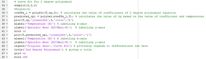
4) The curve fit for 2nd degree polynomial is created, “polyfit” command is used to calculate the values of the coefficients of the polynomial equation and then with “polyval”, the values of “predicted_cp1” is calculated with coefficients and the temperature as an input. This step has to be repeated in order to get the 3rd degree predicted values. So, follow the same steps for 3rd degree of polynomial.

I have here used a subplot command to plot the all the 4 graphs in a single figure window. The subplot command will help us achieve our goal. The (2,2,2) signifies that, it is a (2,2) figure window with 2 being the 2nd subplot. This step has to be repeated for all the polynomial degrees below.

Open a new figure window using “figure” command, with “plot” command plot the original data, and then plot the 1 degree polynomial data. Now for labelling the x – axis and y – axis use “xlabel” and “ylabel” respectively. Lastly, provide legends for differentiating the data by using “legends” command, for giving a title using “title” command. Follow the same steps for 3 degree polynomial data.

5) The curve fit for 3rd degree polynomial is created, “polyfit” command is used to calculate the values of the coefficients of the polynomial equation and then with “polyval”, the values of “predicted_cp1” is calculated with coefficients and the temperature as an input.

I have here used a subplot command to plot the all the 4 graphs in a single figure window. The subplot command will help us achieve our goal. The (2,2,2) signifies that, it is a (2,2) figure window with 3 being the 3rd subplot.

Open a new figure window using “figure” command, with “plot” command plot the original data, and then plot the 1 degree polynomial data. Now for labelling the x – axis and y – axis use “xlabel” and “ylabel” respectively. Lastly, provide legends for differentiating the data by using “legends” command, for giving a title using “title” command.

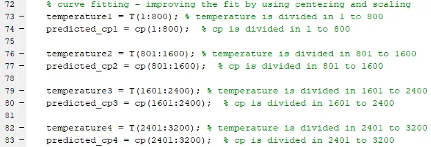
6) I divided the whole data set into 4 parts that is (1 – 800), (801 – 1600), (1601 – 2400), and (2401 – 3200). Now I assigned the values of these individual parts to 4 sets of temperature (with suffix 1, 2, 3, 4) and 4 sets of cp (with suffix 1, 2, 3, 4). This method will help us reduce the bad conditioned characteristics of the polynomial equation.

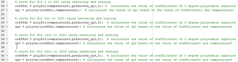
7) Now to get the curve fit we use the “polyfit” command to determine the coefficients of the polynomial and “polyval” command and to calculate the value of cp on the basis of coefficients and temperature which was determined using the polyfit. I have used a 3rd degree polynomial equation here and for that centering and scaling a “polyfit” command is used so that there are no warnings. Output of “polyfit” here is saved in four variables, as the degree of polynomial is therefore it requires four inputs for evaluating the new “cp”.

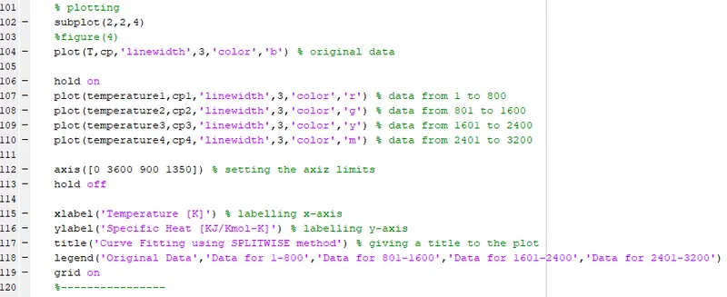
8) Now plot the data using the “plot” command, start with the original data, then using “hold on” command plot the data for the ranges 1 – 800, 801 – 1600, 1601 – 2400, and 2401 – 3200. Now for labelling the x – axis and y – axis use “xlabel” and “ylabel” respectively. Now provide legends for differentiating the data by using “legends” command, for giving a title using “title” command. I will post the answer of this plot in the output section of this report.

Methods of improvement of the cubic fit:

The Step 6 to Step 8 in the programming explaination section above in this report, is one way to improve the quality of the cubic fit.

Errors faced and steps took to overcome:

Did not face any major errors. All the minor errors were corrected as soon as it was evident.

Output:

1. How to make a curve fit perfectly?

To make a curve fit perfectly or get a more robust curve , we can increase the degree of polynomial or use split-wise polynomial that seperates the set of data into two different ranges and are specified to two different variable and then plotted together.

2. What could be done to improve the cubic fit?

To impove the cubic fit, we can use split-wise polynomial that seperates the set of data into two different ranges and are specified to two differetn variables and then plotted together or we can add points with distinct values for x.

3. How to get the best fit?

A best fit plot can be obtained by either making use of centre and scale features in the polyval and polyfit functions. Also, In the Curve Fitting app, we have an option to the select X Data and Y Data. The Curve Fitting app creates a default interpolation whichs fits the data. This tool addon is quick and useful for such problems.

Plots:

References:

• https://projects.skill-lync.com/projects/Curve-Fitting-and-criterion-to-choose-best-fit-41860
• NPTEL lecture of IIT madras.
• Youtube videos on Curve Fitting.