Week 4.1 - Genetic Algorithm
AIM:
Optimisation of a Stalagmite Function Using MATLAB.
OBJECTIVE:
- To optimise the stalagmite function and to find the global maxima of the function.
- To plot the graphs for all the studies of Function Maximum VS Iterations.
GENETIC ALGORITHM:
A genetic algorithm (GA) is a method for solving both constrained and unconstrained optimization problems based on a natural selection process that mimics biological evolution. The algorithm repeatedly modifies a population of individual solutions. At each step, the genetic algorithm randomly selects individuals from the current population and uses them as parents to produce the children for the next generation. Over successive generations, the population "evolves" toward an optimal solution.
You can apply the genetic algorithm to solve problems that are not well suited for standard optimization algorithms, including problems in which the objective function is discontinuous, nondifferentiable, stochastic, or highly nonlinear.
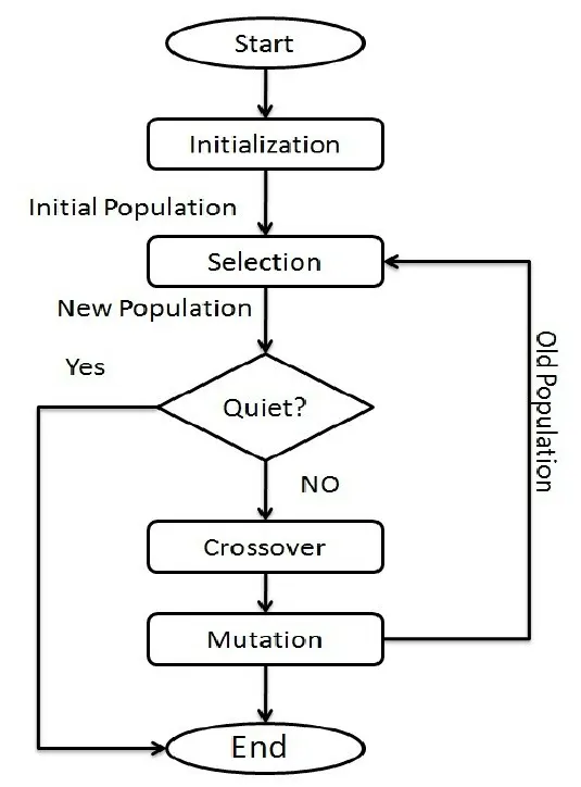
The Genetic Algorithm is Based on the Darwian Theory of evolution proposed by the Charles Darwin.

The genetic algorithm differs from a classical, derivative-based, optimization algorithm in two main ways, as summarized in the following table.
| Classical Algorithm | Genetic Algorithm |
|---|---|
| Generates a single point at each iteration. The sequence of points approaches an optimal solution. | Generates a population of points at each iteration. The best point in the population approaches an optimal solution. |
| Selects the next point in the sequence by a deterministic computation. | Selects the next population by computation which uses random number generators. |
The Evolution Works on the Following Binary Case:
- Selection
- Crossover
- Mutation
STALAGMITE:
A stalagmite function generally refers to the function with which we are generating values over a stalagmite kind of surface for finding out the local and global maxima and minima of that particular given function. For this in Matlab we are using a method called 'Optimization'
OPTIMIZATION:
Optimization is the Process of 'Making Something Better'.
It Refers to the finding the value of the input in order to get the best value for the output, The Definition of the 'best' varies from problem to problem, but in mathematical terms it refers to maximizing or minimizing the input functions , by varying the input parameters.
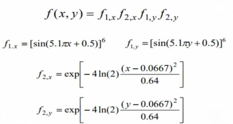
MATLAB CODE FOR STALAGMITE FUNCTION:
function [f] = stalagmite(input)
x = input(1);
y = input(2);
f1x= (sin(5.1*pi*x + 0.5))^6;
f1y= (sin(5.1*pi*y + 0.5))^6;
f2x = exp((-2.7726)*(x-(0.0667))^2/0.64);
f2y = exp((-2.7726)*(y-(0.0667))^2/0.64);
f = -(f1x*f1y*f2x*f2y);
end
GENETIC ALGORITHM SYNTAX:
x = ga(fun,nvars,A,B,Aeq,Beq,lb,ub,nonlcon,intcon,options)
where,
fun = objective function;
nvars = no.of variables;
A & B = subject to linear inequalities of the form A*x<= B;
Aeq & Beq = subject to linear inequalitites of the form A*x=B;
lb= lower bound;
ub = upper bound;
nonlcon = non-linear inequalities;
intcon = interger constrained;
options = helps to add constraint tolerance by increasing the population size;
MATLAB CODE:
%basic stalagmite plot code
clear all
close all
clc
%defining the work space
x = linspace(0,0.6,150);
y = linspace(0,0.6,150);
num_cases = 50;
% creating the 2d plot
[xx yy] = meshgrid(x,y);

%Evaluating the stalagmite function
for i= 1:length(xx);
    for j= 1:length(yy);
        input_vector(1) = xx(i,j);
        input_vector(2) = yy(i,j);
        %function definition.
        f(i,j) = stalagmite(input_vector);
    end
end

%evaluating genetic algorithm evolution
for k=1:num_cases;
    [inp,fval(k)] = ga(@stalagmite,2);
    x_1(k) = inp(1);
    y_1(k) = inp(2);
end
figure(1)
hold on
grid on
surfc(xx,yy,-f)
shading interp
title('stalagmite plot')
xlabel('x')
ylabel('y')
zlabel('f')
RESULTS:
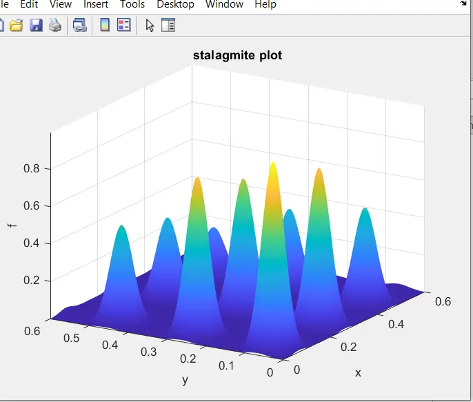
Therefore, We got the basic stalagmite plot and as we see there are so many up-growing peaks,resembles the stalagmite structure. Hence it tends to give the rise of the negative values(Local Minima),we will make the function positive in order to get the local ang Global Maxima.
1. Study_1: [unbounded inputs]:
clear all
close all
clc
%defining the work space
x = linspace(0,0.6,150);
y = linspace(0,0.6,150);
num_cases = 50;
% creating the 2d plot
[xx yy] = meshgrid(x,y);

%Evaluating the stalagmite function
for i= 1:length(xx);
    for j= 1:length(yy);
        input_vector(1) = xx(i,j);
        input_vector(2) = yy(i,j);
        f(i,j) = stalagmite(input_vector);
    end
end


tic
%to study statistical behaviour study_1
for l=1:num_cases;
    [inputs,fopt(l)] = ga(@stalagmite,2)
    x_2(l) = inputs(1);
    y_2(l) = inputs(2);
end
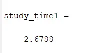
study_time1 = toc
 figure(2)
 subplot(2,1,1)
 surfc(xx,yy,-f)
 shading interp
 hold on
 plot3(x_2,y_2,-fopt,'marker','o','markersize',5,'markerfacecolor','r')
 title('unbounded inputs')
 subplot(2,1,2)
 plot(fopt)
 xlabel('iterations')
 ylabel('function maximum')
RESULTS:
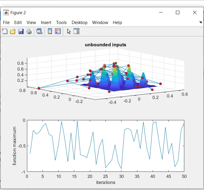
RESULTS
In the above image we can clearly see that the inputs are unbounded, the GA algorithm mapped all possible values of the global maxima outside the stalagmite function. moreover we requite the single global maxima so the case study continued to next stage.
STUDY_2[Bounded inputs]:
clear all
close all
clc
%defining the work space
x = linspace(0,0.6,150);
y = linspace(0,0.6,150);
num_cases = 50;
% creating the 2d plot
[xx yy] = meshgrid(x,y);

%Evaluating the stalagmite function
for i= 1:length(xx);
    for j= 1:length(yy);
        input_vector(1) = xx(i,j);
        input_vector(2) = yy(i,j);
        f(i,j) = stalagmite(input_vector);
    end
end


tic
%to study statistical behaviour with upper and lower bounds
for m = 1:num_cases;
    %objective function is stalagmite and the number of variavles is 2
    %A,B,Aeq,Beq is[],because there is no linear equalities and
    %inequalities
    %lower boundry of the variable X and y are set as [0 ;0]
    %upper boundry of the variable X and y are set as [0.3;0.3]
    [inputs , fopt(m)] = ga(@stalagmite,2,[],[],[],[],[0;0],[0.3;0.3]);
    x_3(m) = inputs(1);
    y_3(m) = inputs(2);
end
study_time2 = toc
 figure(3)
 subplot(2,1,1)
 surfc(xx,yy,-f) %ga gives the minimum value, inverse gives the maximum
 shading interp  %a smooth curve without mesh lines
 hold on
 plot3(x_3,y_3,-fopt,'marker','o','markersize',5,'markerfacecolor','r')
 title('bounded inputs')
 subplot(2,1,2)
 plot(fopt)
 xlabel('iterations')
 ylabel('function maximum')
RESULTS:
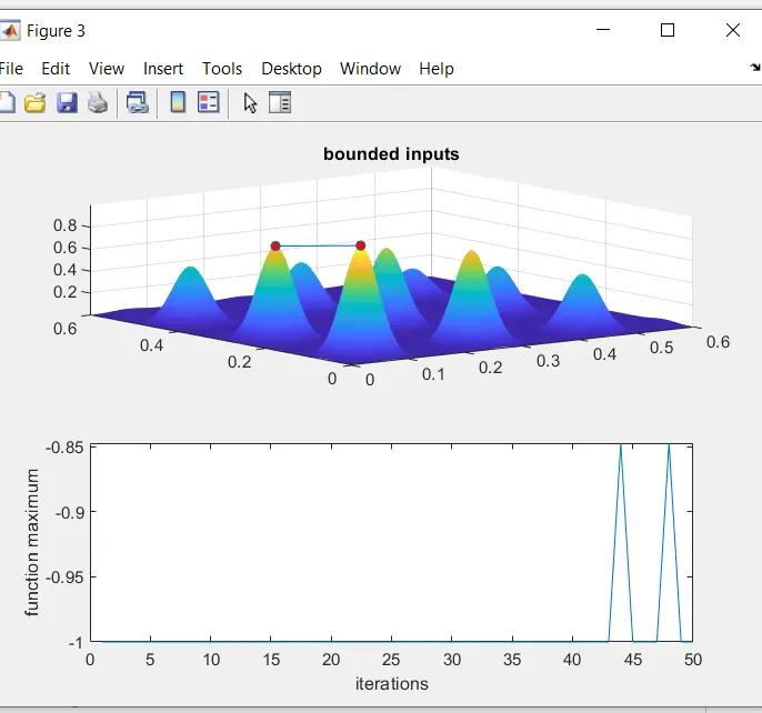
From the above diagram, we have defined the space[limits] for the global maxima , we can also optimize it through to get the perfect solution.
STUDY_3[Bounded inputs with increased population size]:
clear all
close all
clc
%defining the work space
x = linspace(0,0.6,150);
y = linspace(0,0.6,150);
num_cases = 150;
% creating the 2d plot
[xx yy] = meshgrid(x,y);

%Evaluating the stalagmite function
for i= 1:length(xx);
    for j= 1:length(yy);
        input_vector(1) = xx(i,j);
        input_vector(2) = yy(i,j);
        f(i,j) = stalagmite(input_vector);
    end
end
tic
%Incresing GA iterations
options = optimoptions('ga')
options = optimoptions(options,'PopulationSize',450)
for n = 1:num_cases;
    m = 1:num_cases;
    %objective function is stalagmite and the number of variavles is 2
    %A,B,Aeq,Beq is[],because there is no linear equalities and
    %inequalities
    %lower boundry of the variable X and y are set as [0 ;0]
    %upper boundry of the variable X and y are set as [0.3;0.3]
    %options to incease the populationsize
    [inputs , fopt(n)] = ga(@stalagmite,2,[],[],[],[],[0;0],[0.3;0.3],[],[],options);
    x_4(n) = inputs(1);
    y_4(n) = inputs(2);
end
study_time3 = toc
 figure(4)
 subplot(2,1,1)
 surfc(xx,yy,-f) %ga gives the minimum value, inverse gives the maximum
 shading interp  %a smooth curve without mesh lines
 hold on
 plot3(x_4,y_4,-fopt,'marker','o','markersize',5,'markerfacecolor','r')
 title('bounded inputs with incresed population size')
 subplot(2,1,2)
 plot(fopt)
 xlabel('iterations')
 ylabel('function maximum')
RESULTS:
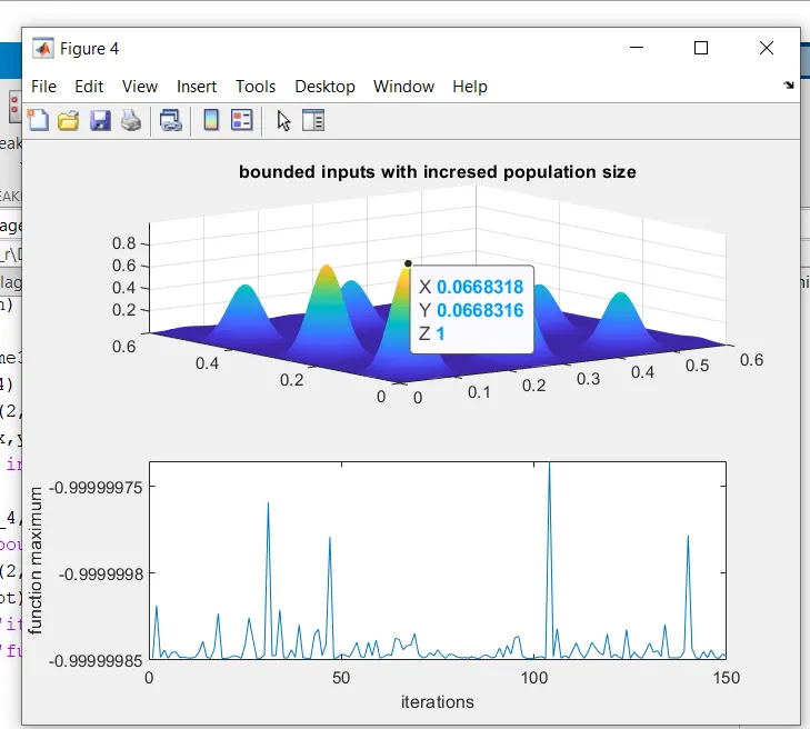
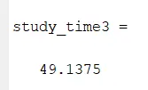
As the above images, denotes the optimised value of the global maxima with accurate range, Since we have increased the no of iterations and the polulation size. so that the study time is 3 times higher than the previous study cases.
CONCLUSION:
Hence we can conclude that GA will give more accurate results with the bounded inputs and the increased popualtion size.