CURVE FIT ANALYSIS
AIM:
To write a code to fit a curve and also usung splitwise method for the same.
THEORY:
Curve fitting is the process of constructing a curve, or mathematical function, that has the best fit to a series data of points, possibly subject to constraints. Curve fitting can involve either interpolation, where an exact fit to the data is required, or smooting, in which a "smooth" function is constructed that approximately fits the data. A related topic is regression analysis, which focuses more on questions of statistical interface such as how much uncertainty is present in a curve that is fit to data observed with random errors. Fitted curves can be used as an aid for data visualization, to infer values of a function where no data are available, and to summarize the relationships among two or more variables. extrapolation refers to the use of a fitted curve beyond the range of the observed data, and is subject to a degree of freedom since it may reflect the method used to construct the curve as much as it reflects the observed data.
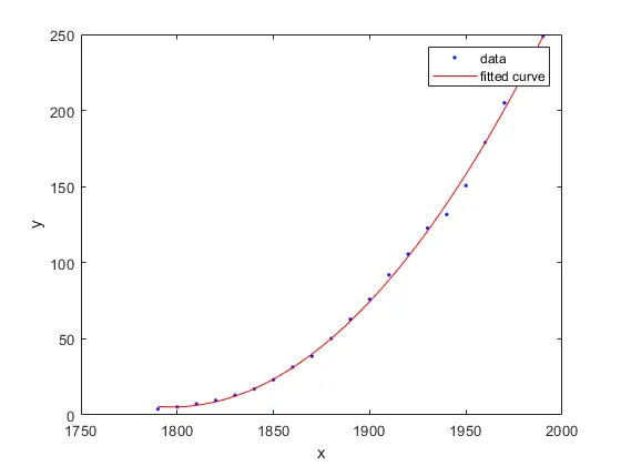
here we are using 3 methods in order to determine the best curve fit:
- linear polynomial curve fitting.
- cubic polynomial curve fitting.
- splitwise method
To understand the goodness of the curve fit we need to calculate the 4 parameters.
- SSE = sum of squares due to error.
- R = relation between response values and predicted values.
- R_Adj = adjacent values of R.
- RMSE = root mean square error.
SSE is sum of squares due to error , it can be calculated as
SSE = (YI-I)^2
SST = total sum of squares
SSR = sum of squares due to regression.
SST = SSR + SSE
R square = SSR/SST
RMSE = `sqrt x`SSE/n
1. Linear polynomial
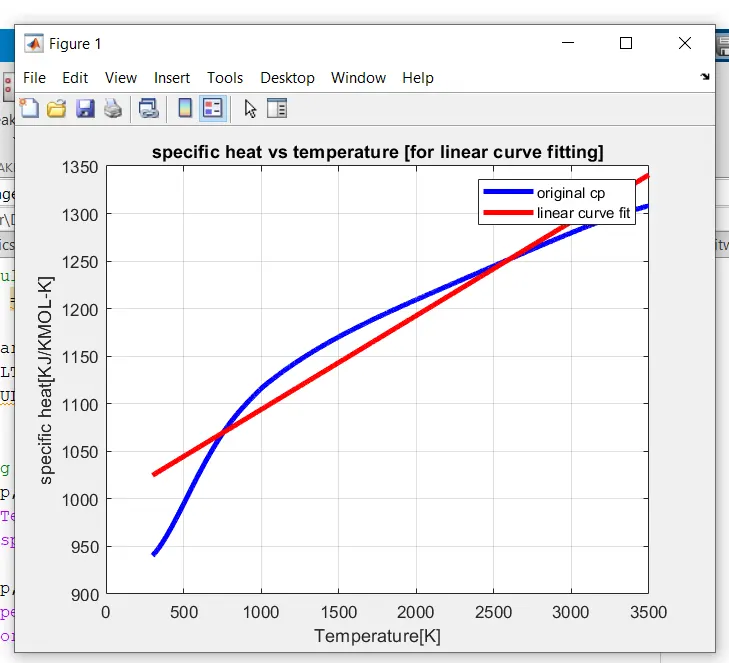
here in linear method, the equation is expressed as;
Y = ax+b, is a straight line with slope a
by using this equation the line can fit two points.
'polyfit' is a MATLAB command that computes the data by least square method. It generates the coefficient of polynomials which is used to fit a curve.
'polyval' is a MATLAB function which evaluates the polynomial with agiven set of data points. It generates the curve to fit a data based on the coefficients calculated by the polyfit function.
CODE:
%program to linear polynomial
clear all
close all
clc
%inputs
cp_data = load('data');
temp = cp_data(:,1);
cp = cp_data(:,2);
%curvefit
%y = a*x + b
coeff= polyfit(temp,cp,1);
predicted_cp = polyval(coeff,temp);
total_cp = 0;
%to calculate the total_cp
for m = 1:length(cp(:,1))
    total_cp = total_cp + cp(m);
end

%to calculate the mean-cp
mean_cp = total_cp/3200;

%to calculate the SSR
SSR = 0;
for n =1:length(cp(:,1))
    SSR = SSR + (predicted_cp(n) - mean_cp).^2;
end
 %to calculate the SSE
 SSE = 0
 for o= 1:length(cp(:,1))
     SSE = SSE + (cp(o) - predicted_cp(o)).^2;
 end
 %to calculate SST
 SST = SSR+SSE;
 %to calculate R_square
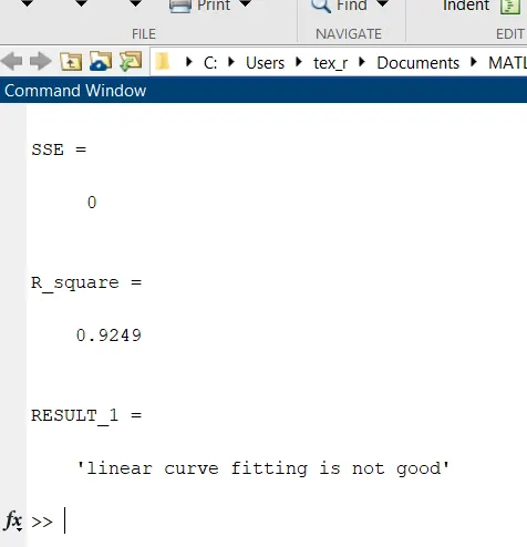
 R_square = SSR/SST
 %print
 if R_square > 0.95
     RESULT_1 = sprintf('linear curve fitting is good')
 else RESULT_1= sprintf('linear curve fitting is not good')

 end
 %plotting
 plot(temp,cp,'linewidth',3,'color','b')
 xlabel('Temperature[K]')
 ylabel('specific heat[KJ/KMOL-K]')
 hold on
 plot(temp,predicted_cp,'linewidth',3,'color','r');
 title('specific heat vs temperature [for linear curve fitting]')
 legend('original cp','linear curve fit')
 grid on
RESULTS:
CUBIC POLYNOMIAL CURVE FITTING:
%program to cubic polynomial fit
clear all
close all
clc
%inputs
cp_data = load('data');
temp = cp_data(:,1);
cp = cp_data(:,2);
%curvefit
%y = a*x^3+b*x^2+c*x+d
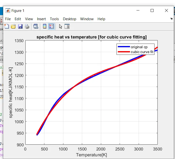
coeff= polyfit(temp,cp,3);  % the degree of the polynomial is 3
predicted_cp = polyval(coeff,temp);
total_cp = 0;
%to calculate the total_cp
for m = 1:length(cp(:,1))
    total_cp = total_cp + cp(m);
end

%to calculate the mean-cp
mean_cp = total_cp/3200;

%to calculate the SSR
SSR = 0;
for n =1:length(cp(:,1))
    SSR = SSR + (predicted_cp(n) - mean_cp).^2;
end
 %to calculate the SSE
 SSE = 0
 for o= 1:length(cp(:,1))
     SSE = SSE + (cp(o) - predicted_cp(o)).^2;
 end
 %to calculate SST
 SST = SSR+SSE;
 %to calculate R_square
 R_square = SSR/SST
 %print
 if R_square > 0.95
     RESULT_2 = sprintf('linear curve fitting is good')
 else RESULT_2= sprintf('linear curve fitting is not good')

 end
 %plotting
 plot(temp,cp,'linewidth',3,'color','b')
 xlabel('Temperature[K]')
 ylabel('specific heat[KJ/KMOL-K]')
 hold on
 plot(temp,predicted_cp,'linewidth',3,'color','r');
 title('specific heat vs temperature [for cubic curve fitting]')
 legend('original cp','cubic curve fit')
 grid on
RESULTS:
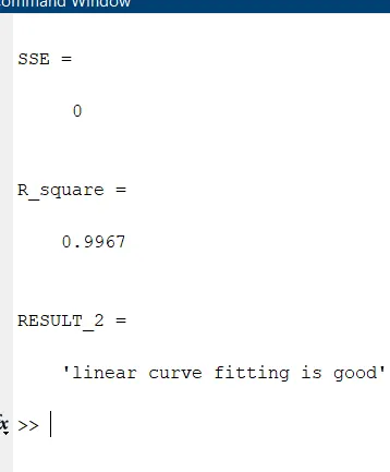
SPLITWISE CURVE FIT:
CODE:
clear all
close all
clc
%inputs
cp_data = load('data');
temp = cp_data(:,1);
cp = cp_data(:,2);
%curve fit
coeff = polyfit(temp,cp,1);
predicted_cp = polyval(coeff,temp);
%plotting
plot(temp,cp,'linewidth',3,'color','b');
xlabel('temperature[K]')
ylabel('specific heat [KJ/KMOL-K]')
hold on
%splitwise method
%1 split
temp1 = cp_data(1:640,1);
cp1 =cp_data(1:640,2);
coeff1= polyfit(temp1,cp1,1);
predicted_cp1 = polyval(coeff1,temp1);
%2 split
temp2 = cp_data(641:1280,1);
cp2 =cp_data(641:1280,2);
coeff2= polyfit(temp2,cp2,1);
predicted_cp2= polyval(coeff2,temp2);
%3 split
temp3 = cp_data(1281:1920,1);
cp3 =cp_data(1281:1920,2);
coeff3= polyfit(temp1,cp3,1);
predicted_cp3 = polyval(coeff3,temp1);
%4 split
temp4 = cp_data(1921:2560,1);
cp4 =cp_data(1921:2560,2);
coeff4= polyfit(temp4,cp4,1);
predicted_cp4 = polyval(coeff4,temp4);
% 5 split
temp5 = cp_data(2561:3200,1);
cp5 =cp_data(2561:3200,2);
coeff5= polyfit(temp5,cp5,1);
predicted_cp5 = polyval(coeff5,temp5);
% examine the goodness of the fit
% to calculate the total cp
total_cp = 0;
for i = 1:640
total_cp1 = total_cp + cp1(i);
total_cp2 = total_cp + cp2(i);
total_cp3 = total_cp + cp3(i);
total_cp4 = total_cp + cp4(i);
total_cp5 = total_cp + cp5(i);
end
% to calculate  the meancp
mean_cp1 = total_cp1/640;
mean_cp2 = total_cp2/640;
mean_cp3 = total_cp3/640;
mean_cp4 = total_cp4/640;
mean_cp5 = total_cp5/640;
% to calculate SSR
SSR = 0;
for j= 1:640
    SSR1 = SSR + (predicted_cp1(j)- mean_cp1).^2;
    SSR2 = SSR + (predicted_cp2(j)- mean_cp2).^2;
    SSR3 = SSR + (predicted_cp3(j)- mean_cp3).^2;
    SSR4 = SSR + (predicted_cp4(j)- mean_cp4).^2;
    SSR5 = SSR + (predicted_cp5(j)- mean_cp5).^2;
end
SSR = SSR1+SSR2+SSR3+SSR4+SSR5;
%to calculate the SSE
SSE = 0;
for k =1:640
    SSE1 =SSE + (cp1(k) - predicted_cp1(k)).^2;
    SSE2= SSE + (cp2(k) - predicted_cp2(k)).^2;
    SSE3= SSE + (cp3(k) - predicted_cp3(k)).^2;
    SSE4= SSE + (cp4(k) - predicted_cp4(k)).^2;
    SSE5= SSE + (cp5(k) - predicted_cp5(k)).^2;
end
SSE = SSE1+SSE2+SSE3+SSE4+SSE5;
%to calculate the SST
SST = SSR+SSE;
% to calculate the r_square
R_square = SSR/SST
%results
if R_square > 0.95
    RESULT3 = sprintf('splitwise curve fitting is good')
else
    sprintf('splitwise curve fitting is not good')
end

%plotting
plot(temp1,predicted_cp1,'linewidth',3,'color','r');
plot(temp2,predicted_cp2,'linewidth',3,'color','r');
plot(temp3,predicted_cp3,'linewidth',3,'color','r');
plot(temp4,predicted_cp4,'linewidth',3,'color','r');
plot(temp5,predicted_cp5,'linewidth',3,'color','r');
title('temperature vs specific heat[for splitwise curve fitting]')
xlabel('temperature [K]')
ylabel('specific heat [KJ/KMOL-K]')
legend('original data','splitwise curve fitting')
grid on
RESULTS:
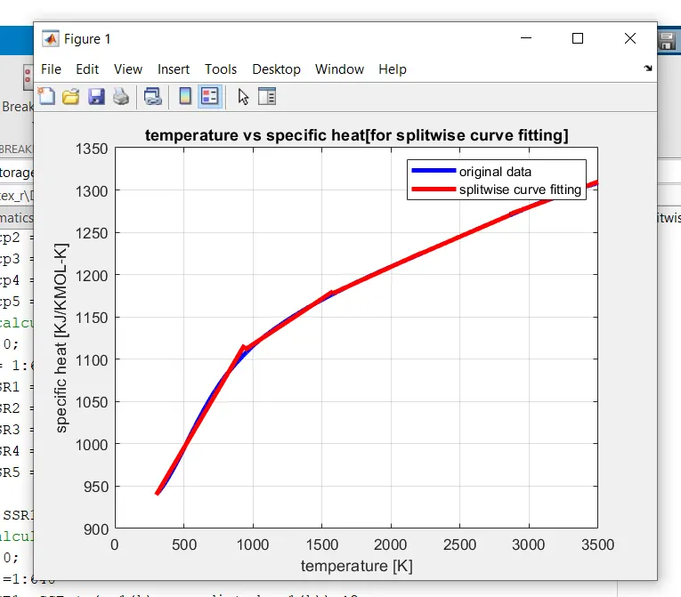
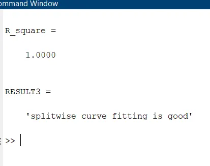
Finally in the splitwise method , the value of the R-square turns to be an unity, which means all the values are represented by SSE.the curve fits almost all the original data and therefore we can declare the goodness of the fit.
QUESTIONS:
1. How to make a prefect curve fit?
Practically, it is not possible to attain the perfect curve, but we can obtain the nearest value without imbalance in the equation.Among many curve fits interpolant method gives us the nearest results.hence it is always a good practice to go with spliiting the data, centering, normalaizing as well.
2.How to get the best fit?
There is diffrence between the best fit and the perfect fit.Best fit means to validate the characteristics of the curveand to minimize the error with in fesible manner, without violating the characteristics of the curve.
Im order to get the best fit,we need to increase the order of the polynomial to a harmless extent or split the data in to the certain fragments and try to fit the curve accordingly.
CONCLUSION:
Hence the curve fit is analyzed for three diffrent parameters.