Week 3 - Solving second order ODEs

AIM:

Solving a Second Order Diffrential Equation for simulate simple pendulum motion using MATLAB .

THEORY:

A simple pendulum is one which can be considered to be a point mass suspended from a string or rod of negligible mass. It is a resonant system with a single resonant frequency. For small amplitudes, the period of such a pendulum can be approximated by: Show. For pendulum length

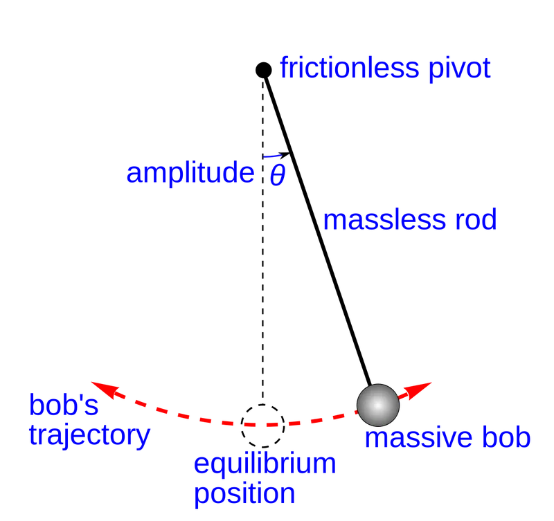
In Engineering, ODE is used to describe the transient behavior of a system. A simple example is a pendulum.The way the pendulum moves depends on the Newtons second law. When this law is written down, we get a second order Ordinary Differential Equation that describes the position of the "ball" w.r.t time.

Similarly, there are hundreds of ODEs that describe key phenomena and if you have the ability to solve these equations then you will be able to simulate any of theses systems.

This ODE represents the equation of motion of a simple pendulum with damping

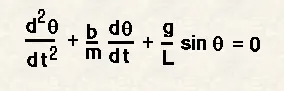
In the above equation,

g = gravity in m/s2,

L = length of the pendulum in m,

m = mass of the ball in kg,

b=damping coefficient.

L=1 metre,

m=1 kg,

b=0.05.

g=9.81 m/s2.

Simulating motion between 0-20 sec, for angular displacement=0,angular velocity=3 rad/sec at time t=0.

MATLAB CODE:

%program to solve a second order diffrential equation for a simple pendulum
clear all
close all
clc

%input parameters
b = 0.05;    %damping co-efficient
g = 9.81;    %gravitational constant
l = 1;        %length of the string
m = 1;       %mass of the bob

% initial condition
theta_0 = [0;3]; %angular dispalcement and velocity

% time
t_span = linspace(0,20,150);   %0-20(150) values in between

% solving the ODE
[t, results] = ode45(@(t,theta)ode_func(t,theta,b,g,l,m),t_span,theta_0);

plot(t,results(:,1)) %plotiing all the values of the dispalcement
figure (1)
hold on
plot(t,results(:,2))   %plotting all the values of the velocity)as
grid on
xlabel('time')
ylabel('plot')
legend(' angular displacement','angular velocity')
title('MOTION OF THE PENDULUM')

 %to create the animation
 
ct = 1; %initial value of the counter to keep track of frame number
for i = 1:length(results(:,1))
    x0 = 0;
    y0 = 0;
    x1 = l*sin(results(i,1));
    y1 = -l*cos(results(i,1));
    
    figure (2)
    plot(x0,y0,'-square','MarkerSize',15,'MarkerFaceColor','r','MarkerEdgeColor','r','color','r') %the pivot of square shape
    hold on
    plot([x0 x1],[y0 y1],'-','MarkerSize',10,'MarkerFaceColor','b','MarkerEdgeColor','b','linewidth',3,'color','b') %plot the length of the string
    plot(x1,y1,'o','MarkerSize',15,'MarkerFaceColor','r','MarkerEdgeColor','r') %plot ball position
    plot([-1 1],[0 0],'linewidth',2,'color','g')   %plot fixed support
    grid on
    hold off
    axis([-2 2 -2.5 2.5])
    pause (0.1)
    M(ct) = getframe(gcf); %getting the figure and saving in an array called M
    ct = ct + 1  
end
movie(M)
videofile = VideoWriter('pendulum_animation_sample.avi','Uncompressed AVI'); %format to save a animation video
open(videofile)  % opems the file
writeVideo(videofile,M)  % writing frames 
close(videofile)  % closes the file

ode_function code:

% second order diffrential equation (calling function)
function [dtheta_dt] = ode_func(t,theta,b,g,l,m)
theta1 = theta(1)
theta2 = theta(2)
dtheta1_dt = theta2;
dtheta2_dt = -(b/m)*theta2-(g/l)*sin(theta1);
dtheta_dt = [dtheta1_dt;dtheta2_dt];
end

RESULT:

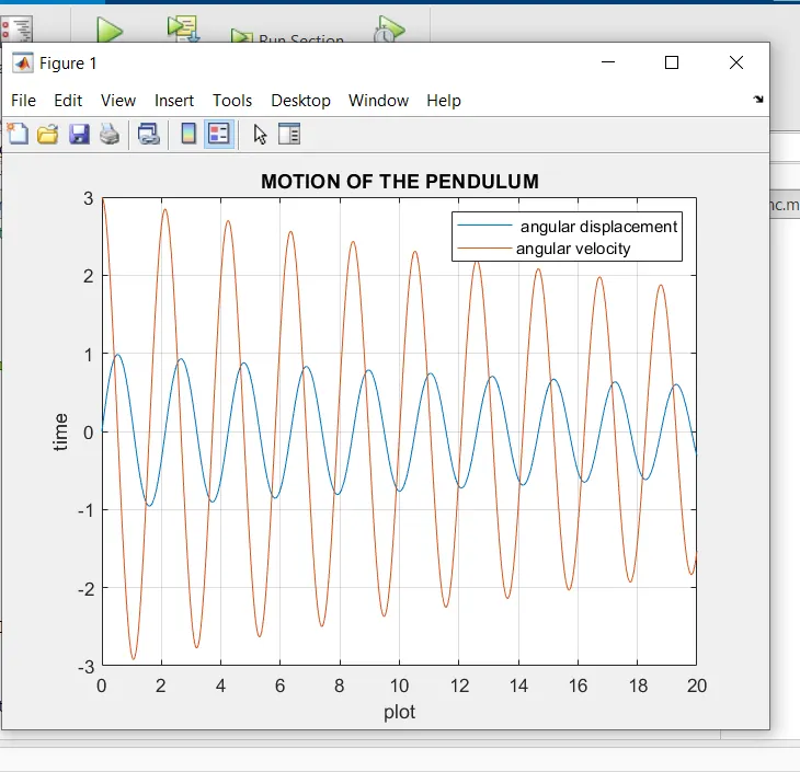
ANIMATION VIDEO LINK:

https://drive.google.com/file/d/1bWyr4tdz8VDSPj4jYldMWosqVffxJdzw/view?usp=sharing

youtube video link: https://youtu.be/nfKZIsnzUvk

APPLICATIONS:

• Pendulums have many applications and utilized often before the digital age.

They were used in clocks and metronorms due to their regularity in time period in wrecking balls, playground swings due to their simple way of building and keeping energy.

CONCLUSION:

Hence the simple pendulem animation is done using ordinary diffrential equation.