Week 4.1 - Genetic Algorithm

AIM: 1. To write a code in MATLAB to optimise the Stalagmite function and find the global maxima of the function.

2. Explain the concept of Genetic Algorithm along with the syntax for ga(genetic algorithm) in MATLAB.

3. To plot graphs for all 3 case studies and plot 'F maximum vs No. of Iterations '. Titles and axes labels a must.

The full Code :

clear all
close all
clc

% Defining Input variables
x = linspace(0,0.6,150);
y = linspace(0,0.6,150);


% Creating a 2Dimensional mesh
[xx,yy] = meshgrid(x,y);

% Evaluating the stalagmaite function
for i = 1:length(xx)
    for j = 1:length(yy)
        input_vector(1) = xx(i,j);
        input_vector(2) = yy(i,j);
        f(i,j) = stalagmite_function(input_vector);
    end
end


% Case 1 study - Unbounded GA
num_case = 50;

tic
for k = 1:num_case
    [inputs1,fopt1(k)] = ga(@stalagmite_function,2);
    xopt1(k) = inputs1(1);
    yopt1(k) = inputs1(2);
end
time1 = toc;

figure(1)
subplot(2,1,1)
hold on
surfc(xx,yy,-f)
shading interp
plot3(xopt1,yopt1,-fopt1,'marker','o','markersize',5,'MarkerFaceColor','r')
title('Unbounded GA')
subplot(2,1,2)
plot(-fopt1)
xlabel('Iterations')
ylabel('Function Maximum')

% Case 2 study - Bounded GA
num_case = 50;

tic
for k = 1:num_case
    [inputs2,fopt2(k)] = ga(@stalagmite_function,2,[],[],[],[],[0;0],[0.4;0.4]);
    xopt2(k) = inputs2(1);
    yopt2(k) = inputs2(2);
end
time2 = toc;

figure(2)
subplot(2,1,1)
hold on
surfc(xx,yy,-f)
shading interp
plot3(xopt2,yopt2,-fopt2,'marker','o','markersize',5,'MarkerFaceColor','r')
title('Bounded GA')
subplot(2,1,2)
plot(-fopt2)
xlabel('Iterations')
ylabel('Function Maximum')

% Case 3 study - Bounded with a Population size
num_case = 50;

options = optimoptions('ga')
options = optimoptions(options,'PopulationSize',300)

tic
for k = 1:num_case
    [inputs3,fopt3(k)] = ga(@stalagmite_function,2,[],[],[],[],[0;0],[0.4;0.4],[],[],options);
    xopt3(k) = inputs3(1);
    yopt3(k) = inputs3(2);
end
time3 = toc;

figure(3)
subplot(2,1,1)
hold on
surfc(xx,yy,-f)
shading interp
plot3(xopt3,yopt3,-fopt3,'marker','o','markersize',5,'MarkerFaceColor','r')
title('Bounded GA with Population Size')
subplot(2,1,2)
plot(-fopt3)
xlabel('Iterations')
ylabel('Function Maximum')

Explanation : We start with clear all, close all, clc. Next step is to define the input variables x and y by using linspace command. The range for x and y is from 0 to 0.6 with a total of 150 values each.

since we have to create a surface plot we have to convert the x and y vector array into 2d array using meshgrid.

Next step is to determine and then store all the output variable in the workspace . Also all the values of input variables x and y have to be stored. For this we use a nested 'for loop'. so that for each and every iteration of y we get a iteration value of x. ie. for 150 values of y we get 150 values of x. The iterations for x and y are denoted by i and j respectively. And for every value of i and j we get values for the Stalagmite function ' f ' .

The code for the Stalagmite function is shown below.

function [f] = stalagmite_function(V)
x = V(1);
y = V(2);

f1x = (sin((5.1*pi*x)+0.5)).^6;
f1y = (sin((5.1*pi*y)+0.5)).^6;
f2x = exp(-4*log(2)*(((x - 0.0667).^2)/0.64));
f2y = exp(-4*log(2)*(((y - 0.0667).^2)/0.64));

f = -(f1x*f1y*f2x*f2y);
end

Case 1 Study - Unbounded GA :

% Case 1 study - Unbounded GA
num_case = 50;

tic
for k = 1:num_case
    [inputs1,fopt1(k)] = ga(@stalagmite_function,2);
    xopt1(k) = inputs1(1);
    yopt1(k) = inputs1(2);
end
time1 = toc;

figure(1)
subplot(2,1,1)
hold on
surfc(xx,yy,-f)
shading interp
plot3(xopt1,yopt1,-fopt1,'marker','o','markersize',5,'MarkerFaceColor','r')
title('Unbounded GA')
subplot(2,1,2)
plot(-fopt1)
xlabel('Iterations')
ylabel('Function Maximum')

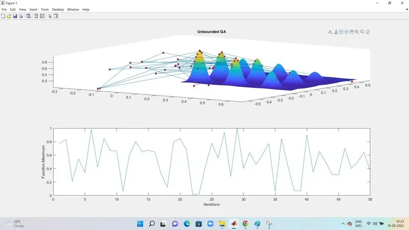
In this case the lower bounds(lb) and upper bounds(ub) are not defined. Hence the data set of points is taken randomly. we have given the number of iterations(num_case) as 50.

The syntax for GA here is :

x = ga(@stalagmite_function,nvars)

Here we perform the ga calling of the stalagmite function. And store values of x , y and the function f values for every iteration. 2 is the number of variables(x and y - nvars).

In order to determine the time taken to study the ga case we use the tic and toc command.

Now , we do the plotting. We use figure(1) to show the case study 1.

We use subplot command to 2 plots in the same figure/window. The first subplot is for surface and stalagmite function. surfc command is used for a surface plot with contour. shading interp command is used to make smooth transition of color from one cell to another and it also inturn will disappear the grid lines showing on the surface. plot3 command is used to plot the optimum values of x,y and f over the 50 iterations.

The second subplot will plot the optimum values that the function is predicting as a function of the iteration.

Below is the picture of the plots in figure(1).

Case 2 Study - Bounded GA :

% Case 2 study - Bounded GA
num_case = 50;

tic
for k = 1:num_case
    [inputs2,fopt2(k)] = ga(@stalagmite_function,2,[],[],[],[],[0;0],[0.4;0.4]);
    xopt2(k) = inputs2(1);
    yopt2(k) = inputs2(2);
end
time2 = toc;

figure(2)
subplot(2,1,1)
hold on
surfc(xx,yy,-f)
shading interp
plot3(xopt2,yopt2,-fopt2,'marker','o','markersize',5,'MarkerFaceColor','r')
title('Bounded GA')
subplot(2,1,2)
plot(-fopt2)
xlabel('Iterations')
ylabel('Function Maximum')

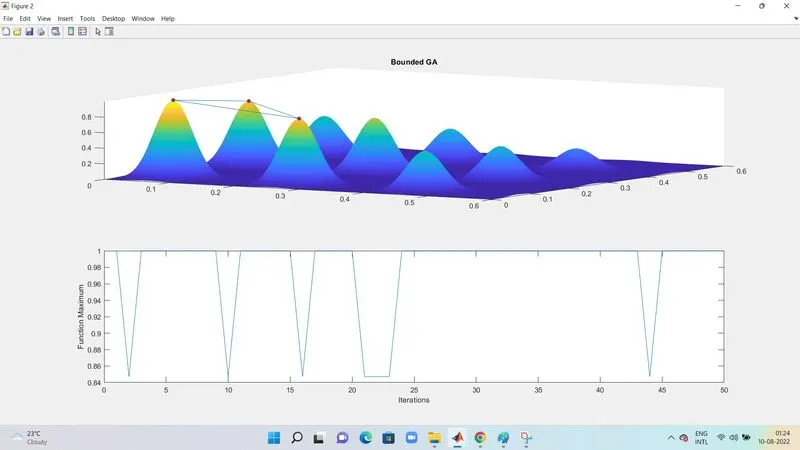
In this case study the lower bounds(lb) and the upper bounds(ub) are defined. And again the num_case is taken as 50.

The GA syntax here is :

x = ga(@stalagmite_function,2,[],[],[],[],[0;0],[0.4;0.4])

The '[]' blank brackets are the place of the linear constraints. They are kept blank as we have not provided any constraints/conditions for the problem. Here the lower bounds for x and y is 0 and the upper bounds for x and y are 0.4 for both. Hence the ga will be performed only within this range.

The output here gives a cleaner and better picture as the function predicts that the maximum point is between 3 points , as shown in the 1st subplot.

Below is the picture of the plots in figure(2).

Case 3 Study - Bounded GA with population size :

% Case 3 study - Bounded with a Population size
num_case = 50;

options = optimoptions('ga')
options = optimoptions(options,'PopulationSize',300)

tic
for k = 1:num_case
    [inputs3,fopt3(k)] = ga(@stalagmite_function,2,[],[],[],[],[0;0],[0.4;0.4],[],[],options);
    xopt3(k) = inputs3(1);
    yopt3(k) = inputs3(2);
end
time3 = toc;

figure(3)
subplot(2,1,1)
hold on
surfc(xx,yy,-f)
shading interp
plot3(xopt3,yopt3,-fopt3,'marker','o','markersize',5,'MarkerFaceColor','r')
title('Bounded GA with Population Size')
subplot(2,1,2)
plot(-fopt3)
xlabel('Iterations')
ylabel('Function Maximum')

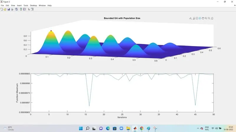
In this case study the lower bounds(lb) and the upper bounds(ub) are defined. Also the population size here is taken as 300. And again the num_case is taken as 50.

The GA syntax here is :

x = ga(@stalagmite_function,2,[],[],[],[],[0;0],[0.4;0.4],[],[],options)

The '[]' blank brackets are the place of the linear and the non linear constraints. The first 4 blank brackets are for linear constraints and the other 2 blank brackets are for non linear constraints. They are kept blank as we have not provided any constraints/conditions for the problem.

Conclusion :

1. Case study 1: After plotting of the Stalagmite function and then the maximum values that the ga is trying to predict, we can see that because of random sampling the points/population are scattered because ga is not having a boundary/range. This gives highly inaccurate results and the output tends to be unstable.

2. Case study 2 : Here the plot will have a better and a cleaner look. In this figure ,the first plot shows that the function predicts that the maximum point is betweeen the 3 points. Which is much better than the previous plot. Also , the variation here is less and the maximum values are between a much lesser range here compared to the previous case 1. But , it is still not very accurate. Lower range will give a better accuracy.

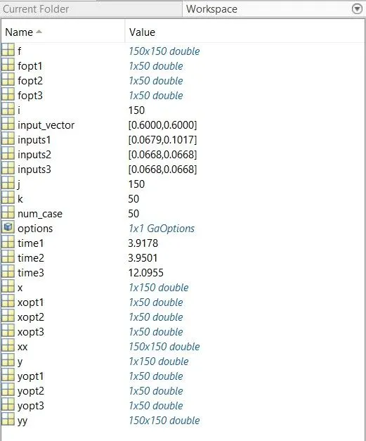
3. Case study 3 : By default ga solver takes the population size as 50. but here we have taken the population size as 300. The search range will remain the same as case 2 study ie 0 to 0.4. Increasing the population size with the same range will give a accurate result of maximum point. Increasing the population size will increase the simulation time as then number of samples are more . hence more time in processing.

Below is the screenshot of the workspace.

Errors :

1. Use of iteration ' i ' in all the for loops. In the workspace the value of ' i ' was showing as 50 instead of 150. The variable ' k ' is used instead of ' i ' in the for loops of case studies.

2. Use of the variable name as input instead of inputs. Which will give a n error of unrecognized variable input.

3. In the surface plots the sign of the stalagmite function f has to be given -ve in this problem , as it will give the the surface plot of minima instead of the requirement of Maxima in the problem.

Concept of Genetic Algorithm : In order to understand the concept of Genetic Algorithm , we have to first understand what is Optimization . Optimization is the process of selection from the set of values and getting the best results/output from the values under a set of prioritized criteria or constraints. It is a procedure which is executed iteratively by comparing various solutions till an optimum solution is found.

Some of the applications of Optimization include ,

1. Mechanics

2. Economics and finance.

3. Machine learning.

4. Artificial intelligence.

5. Controls Engineering.

Flow Chart for the optimization process :

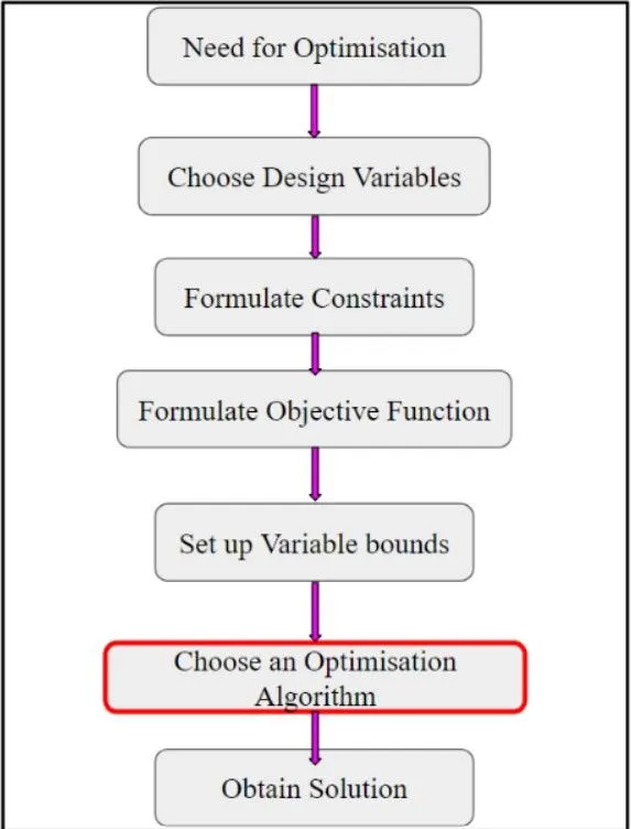
We need to choose an optimization algorithm to perform the optimization process. Genetic Algorithm is that process. In other words , Genetic Algorithm is the study of the process of Optimization.

Flowchart explaining the working of Genetic Algorithm:

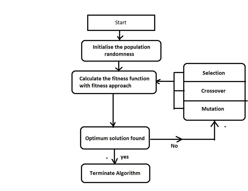
The 3 main processes going behind the GA solvers are :

1. Selection : It is defined as the selection of parents for the next generation using selection function/fitness function which will be based on the fitness value.

2. Crossover : Crossover enables the algorithm to extract the best characteristics from different individuals and recombine them into potentially superior children.

3. Mutation : Mutation adds to the diversity of a population and therby increases the likelyhood that the algorithm will generate individuals with better fitness values.

Based on the above processes the types of children produced for next generation from the current population parents is as follows.

a) Elite Child : Individuals having best fitness values.

b) Crossover child : Created by combining the parents.

c) Mutation child : Created by doing random changes to a single parent.

The GA Syntax is mentioned below.

X = ga(fun , nvars , A , b , Aeq , beq , lb , ub , nonlcon , options)

References : Article by Gopinath - GENETIC ALGORITHM explained!! in the FAQ.