Week 3 - Solving second order ODEs
AIM : 1. To write a program to Simulate the Pendulum motion.
2. To create an image that will represent the position of the Pendulum.
3. Animate the motion of Pendulum.
4. Upload the Animation on YouTube.
Description : As already mentioned , the 2nd order ODE(below) , which is based on the Newtons Second Law of motion, represents the equation of motion of a simple pendulum with damping. The equation describes the position of the ball/bob w.r.t Time.
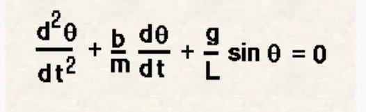
The Input values taken are as below ,
1. b = 0.05 , Damping coefficient.
2. g = 9.81 m/s2 , gravity.
3. l = 1 m , Length of the Pendulum.
4. m = 1 kg , mass of the ball/bob.
5. Time span = 0 to 20 seconds.
6. At time t = 0 ,
a) Angular displacement = 0 rad .
b) Angular velocity = 3 rad/sec .
clear all
close all
clc

% Motion of a simple Pendulum with damping
% Input Values
b = 0.05; % Damping coefficient
g = 9.81; % gravity in m/s2
l = 1;    % Length of the pendulum in m
m = 1;  % mass of the ball in kg

% Time span
t_span = linspace(0,20,250);

% Initial conditions
theta0 = [0;3]; % At time , t = 0

% Solving the ODE
[t,results] = ode45(@(t,theta) Pendulum_motion_function(t,theta,b,g,l,m),t_span,theta0);

y = results(:,1); % Output Values of Angular displacement

figure(1)
plot(t,results(:,1))
hold on
plot(t,results(:,2))
xlabel('Time')
ylabel('Angular displacement/Angular velocity')
legend('Angular displacement','Angular velocity')
grid on

ct = 1;
for i = 1:length(y)     % i = 1:length(results(:,1))
    Y = y(i);

    % Defining the Pendulum pivot point
    x0 = 0;
    y0 = 0;

    % Point at the Pendulum bob
    x1 = l*sin(y(i));
    y1 = -l*cos(y(i));

    % Line 2-3 to which pivot point is connected
    x2 = -1;
    y2 = 0;

    x3 = 1;
    y3 = 0;

    figure(2)
    plot([x0 x1],[y0 y1],'marker','o','LineWidth',2,'color','b')
    hold on
    plot(x1, y1,'marker','o','markersize',20,'markerfacecolor','r','LineWidth',2)
    hold off
    hold on
    plot([x2 x3],[y2 y3],'linewidth',4,'color','m')
    hold off
    title('Pendulum Motion')
    axis([-1.5 1.5 -1.5 1.5])
    pause(0.01)
    M(ct) = getframe(gcf);
    ct = ct + 1;

end

movie(M)
videofile = VideoWriter('Pendulum using 2nd oder ODE.avi')
open(videofile)
writeVideo(videofile,M)
close(videofile)
The time span of 0(start time) to 20(end time) seconds is distributed into 250 values using the linspace command. The initial conditions are represented as a column vector which contains Angular Displacement at the start and Angular Velocity at the start.
To solve the program we use the command ode45 which will be used to solve a 1st order ODE. For that ,the 2nd order ODE equation of motion will be broken down into smaller 1st order ODE's and these 1st order ODE's will be represented by a column vector. The function program will get all the sequence and column vector into a single program.
The function command allows to reuse a set of commands by storing them as a program file.
ode45 command will integrate the system of differential equations using the initial conditions at the initial time till the end time of the time span ' t_span'.
Function program used is shown below.
function [dtheta_dt] = Pendulum_motion_function(t,theta,b,g,l,m)
theta1 = theta(1)  % Angular displacement,theta1 = 0 rad
theta2 = theta(2)  % Angular velocity,theta2 = 3 rad/sec
dtheta1_dt = theta2;
dtheta2_dt = -(b/m)*theta2 -(g/l)*sin(theta1);
dtheta_dt = [dtheta1_dt;dtheta2_dt];
end
Image/graph representing the pendulum motion :
After execution of the ode45 command we get the values as shown below.
Please note : Only few values out of the 250 values are shown. Below image will show only few values of Angular displacement and Angular displacement from the 'results'.
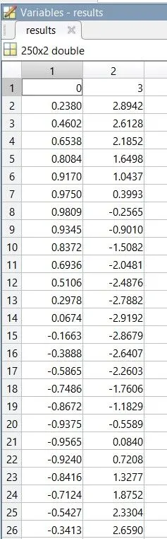
where , in the image shown above , the Angular displacement values are shown in the column 1 and the Angular velocity values are shown in the column 2.
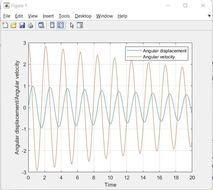
Next , we plot all the 250 values each of Angular displacement and Angular velocity. This graph will be figure(1). figure command is used if we have to show more than one graph/plot at the same time.
The first plot command ie plot(t,results(:,1)) is used to plot the values of Angular displacement by extracting only the Angular displacement values.
Next plot command ie plot(t,results(:,2)) is used to plot the values of Angular velocity by extracting only the Angular velocity values. The hold on command is used so that both the plot commands will be executed otherwise only the last plot command will be displayed. xlabel and ylabel command will show the 'Time' in x axis and 'Angular displacement/Angular velocity' on y axis respectively.
The 'legend' command is used to show the plot representing each plotted data set since there are two different variables in the y axis. 'legend' will differentiate the plot values of Angular displacement from Angular velocity. The grid on commnad will switch on the grid. Please find below the plot showing Angular displacement/Angular velocity vs Time.
Animation of the Pendulum motion :
We use the 'for loop' for this command. The pendulum will be having different angular positions from the start time till the end time. Since there will multiple values of Angular displacement , we will have to repeat the program again and again.
We have taken 'y' as the variable to represent only the Angular displacement values ie. y = results(:,1).
The first line will indicate the length of Angular displacement ie 250 values. So this process will be repeated 250 times. Next, we determine the pivot positon of the pendulum , the point on the pendulum and the line on which the pivot point is connected . Next , we do the plotting. This will be shown as figure(2). First we plot the line from the pivot point (x0,y0) to the Pendulum(x1,y1). Then we use hold on command to plot showing the Pendulum bob/ball. we use hold off command to terminate the the hold on command. Now, we have to plot the line on which the pivot point is connected. we again use hold on and hold off command since this line has to be plotted separately in the same figure.
The title command is used to give a title to the figure. Axis command will show the range of axis to get a better view of the animation. pause command will give a pause between each frame.
Converting the plots into a movie :
The command M(ct) = getframe(gcf) is used to save each and every frame including the first frame and subsequent frames. The number of frames will depend on the number of values of Angular displacement ie. 250 values. Hence to create a movie all these frames have to be joined/stitched together.
The ct command is the counter command and ct = ct +1 will increase the counter ,by 1 , after each frame is saved and the process will go on till the desired condition is reached.
To convert into a movie file or .avi file , we give the following commands.
movie(M)
videofile = VideoWriter('Pendulum using 2nd oder ODE.avi')
open(videofile)
writeVideo(videofile,M)
close(videofile)
After the execution of the full program an .avi file is saved in the same folder as the program file folder and should be named based on the name of program. Here the .avi file will be saved in the compressed form since we have not given 'Uncompressed AVI ' command . After executing the program the animated plot is shown in the output figure followed by the animation movie of the same plot.
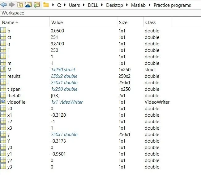
Workspace :
Errors faced during writing of the program :
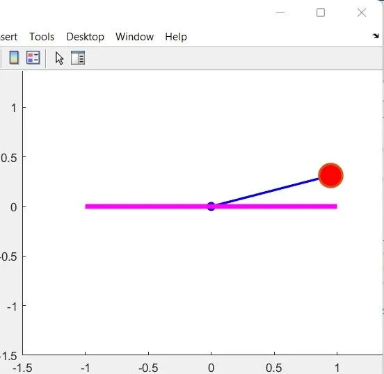
1. Writing incorrect equation(s) for the points x1 and y1 as shown below.
x1 = l*cos(y(i));
y1 = -l*sin(y(i));
The above equations is wrong , since Angular values are taken w.r.t negative y axis. The animation will still work , but will not be correct. see image below.
The correct equations are,
x1 = l*sin(y(i));
y1 = -l*cos(y(i));
The correct animation will work with these equations.
2. Incorrect axis coordinate values in the axis command. The sequence and the signs of values should be correct remembering that the pendulum will be shown in the 3rd and 4th quadrant.
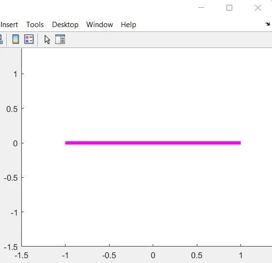
3. The plot for line joining point (x2,y2) and (x3,y3) should be used with hold on and hold off command. Not using these command will only show the last plot command in the program ie it will show only the line 2-3.
Conclusion : The link to the animation is given below.
1. You Tube link :
2. Google Drive link :
https://drive.google.com/file/d/1A0NoutH47bwvIR9_NBZYhVOIHcGAsnQu/view?usp=sharing