Week 4.1 - Genetic Algorithm

Aim: - Perform a Genetic Algorithm study on the stalagmite function of 3 case studies and plot the graph for all 3 cases.

Objective: -

1. Write a code in MATLAB to optimize the stalagmite function and find the global maxima of the function.
2. Clearly explain the concept of genetic algorithm in your own words and also explain the syntax for ga in MATLAB in your report.
3. Make sure that your code gives the same output, even if it is made to run several times.
4. Plot graphs for all 3 studies and for F maximum vs no. of iterations. Title and axes labels are a must, legends could be shown if necessary.

Stalagmite Function governing equation:-

`f(x,y)={[sin(5.1pix+0.5)]^6}*{[sin(5.1pixy+0.5)]^6}*{exp[-4ln(2)((x-0.0667)^2/0.64]}*{exp[-4ln(2)((y-0.0667)^2/0.64]}`

where,

f(x,y) = f is a function of x and y coordinates points.

Theory: -

1. Genetic Algorithm: - it is a global optimization procedure that uses an analogy of the genetic evolution of biological organisms. In other words, genetic algorithms tend to find the best solution to a problem ( Maxima or Minima ) by following an evolutionary process as per our desire.

2. Concept of GA flow chart:-

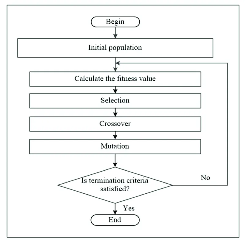
• The GA process begins and initializes the population randomness.
• Calculate the fitness value which has 3 sub-processes as mentioned below-

i) Selection of the points as a parent which is performed on the basis of their fitness level.

ii) After selection, a crossover process extracts the best characters from different points and recombines them into potentially superior children compared to parents.

iii) Mutation is related to the diversity of the points (population) due to the diversity in the population GA can generate points with better fitness values.

• With the help of selection, crossover, and mutation GA will generate the new generation, and the new generation will have a lesser population compared to the previous generation and this will be repeated until GA achieves the maxima point.
• Is termination criteria satisfied (achieve the maxima) if no then GA will repeat the 2nd step until it finds the global maxima.
• After the termination condition is satisfied the GA process comes to an end.

3. Explanation of GA syntax: -

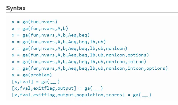
Where,

X, fval = it is an output where X contains the values of (x,y) coordinates and fval contains the optimized function value.

ga = predefined genetic algorithm function name.

fun = this is an objective function (user-defined) which in our case is a stalagmite function.

nvars = number of variables as an input to the ga

A,b = Linear inequality constraints

Aeq,beq = Linear equality constraints

Lb,ub = Lower bounds and upper bounds. These are the boundaries allocated to the ga that mean ga can only be operated within the defined boundaries in x,y axis.

nonlcon = Nonlinear constraints

options = Optimization options that help to change the population size of ga.

In our problem, we have 3 cases where,

1st case unbounded GA study on stalagmite uses: -

[x,fval] = ga(fun,nvars)

In case 1 there are no boundaries for ga to run so it takes the random points from outside of the global boundaries which are not accurate and doesn't help us to achieve our target.

2nd case bounded GA study on stalagmite uses: -

[x,fval] = ga(fun,nvars,A,b,Aeq,beq,lb,ub)

In case 2 we provided the boundaries for ga to run within these boundaries that are lower and upper boundaries this will help us to get closer to our target maxima but still, there are some inaccuracies due to less no. of the population so that is why we will go for case 3 as mentioned below.

3rd case bounded with population size GA study on stalagmite uses: -

[x,fval] = ga(fun,nvars,A,b,Aeq,beq,lb,ub,nonlcon,options)

This is the last case 3 for our problem where we provided the boundaries to the ga and this time we also provided with user-defined population size within the boundaries of ga so this will help to achieve the exact target maxima due to the increase in the population size.

4. Stopping criteria of GA: -

There are certain stopping criteria that are used to stop the GA as follows-

i) Max Generations - when the GA reaches the no. of generations equal to max generations the GA stops.

ii) Max Time - the GA stops running after the specified time in seconds value reaches.

iii) Fitness Limit - the GA stops when the value of the fitness function for the best point in the current population is less than or equal to the fitness limit.

In the below three stopping criteria, one thing is common that there is no or close to no relative change in fitness function value

iv) Max Stall Generations - the GA stops when the average relative change in the fitness function value over Max stall generation is less than function tolerance.

v) Max stall time - the GA stops if there is no improvement in the objective function during an interval of time in seconds.

vi) Function Tolerance - The GA runs until the average relative change in the fitness function value over Max stall generations is less than the function.

5. The significance of running multiple iterations is to cross-check whether the GA is working fine or not, in other words, to check the correctness of the GA. If we run GA 50 times and the maxima values are the same or very close to the same values on each iteration then we can say that the GA is correct.

Stalagmite function code script: -

function [f]= stalagmite(input)
x=input(1);
y=input(2);

f1x=(sin((5.1*pi*x)+0.5))^6;
f1y=(sin((5.1*pi*y)+0.5))^6;
f2x=exp(-4*log(2)*(((x-0.0667)^2)/0.64));
f2y=exp(-4*log(2)*(((y-0.0667)^2)/0.64));

f=-(f1x*f1y*f2x*f2y);
end

GA code main code script: -

clear 
close
clc

%defining the space for GA in x and y.
x = linspace(0,0.6,150);
y = linspace(0,0.6,150);

%Using nested for loop for x and y axis respectively to calculate the stalagmite function f at every point of (x,y).
for i= 1:length(x)
    for j=1:length(y)
        input(1)=x(i);
        input(2)=y(j);
        f(i,j)=stalagmite(input);
    end
end

%Unbounded GA study on the stalagmite function CASE 1.
num_GA_study=50;
for z=1:num_GA_study
    [inputs,fopt(z)]= ga(@stalagmite,2); %here the 'fopt' is the optimized value of the 'f' function and 'inputs' contains x and y optimzed values.
    xopt(z)= inputs(1);
    yopt(z)= inputs(2);
end

figure(1);
subplot(2,1,1)    %supplot command is used to divide the same fig into to sections and plot 2 graphs in it.
surf(x,y,-f);
xlabel('x values')
ylabel('y values')
zlabel('f values')
title('Unbounded GA study')
shading interp   %shading interp is to make the surf looks clean and smooth by removing the lines over it.
hold on
plot3(xopt,yopt,-fopt,'Marker','o', MarkerSize=5, MarkerFaceColor='r');   % 'plot3' command is used to plot the points in 3D space.
subplot(2,1,2)
plot(-fopt)
xlabel('No. of iterations')
ylabel('function maximum value')
grid on

%Bounded GA study on the stalagmite function CASE 2.
for z=1:num_GA_study
    %defines a set of lower and upper bounds on the design variables.
    [inputs,fopt(z)]= ga(@stalagmite,2,[],[],[],[],[0;0],[0.4;0.4]);
    xopt(z)=inputs(1);
    yopt(z)=inputs(2);
end

figure(2);
subplot(2,1,1)    %supplot command is used to divide the same fig into to sections and plot 2 graphs in it.
surf(x,y,-f);
xlabel('x values')
ylabel('y values')
zlabel('f values')
title('bounded GA study case 2')
shading interp   %shading interp is to make the surf looks clean and smooth by removing the lines over it.
hold on
plot3(xopt,yopt,-fopt,'Marker','o', MarkerSize=5, MarkerFaceColor='r');   % 'plot3' command is used to plot the points in 3D space.
subplot(2,1,2)
plot(-fopt)
xlabel('No. of iterations')
ylabel('function maximum value')
grid on
      
%Bounded GA study on the stalagmite function with a population size of 270 CASE 3.
for z=1:num_GA_study
    %defines a set of lower and upper bounds on the design variables with a change in populatio size.
    options = optimoptions('ga'); %returns a set of default options for the SolveName solver.
    options = optimoptions(options,'PopulationSize',270);

    % takes the values of options and solves ga in the required population.
    [inputs,fopt(z)]= ga(@stalagmite,2,[],[],[],[],[0;0],[0.4;0.4],[],[],options);
    xopt(z)=inputs(1);
    yopt(z)=inputs(2);
end

figure(3);
subplot(2,1,1)    %subplot command is used to divide the same fig into to sections and plot 2 graphs in it.
surf(x,y,-f);
xlabel('x values')
ylabel('y values')
zlabel('f values')
title('bounded inputs with population size case 3')
shading interp   %shading interp is to make the surf looks clean and smooth by removing the lines over it.
hold on
plot3(xopt,yopt,-fopt,'Marker','o', MarkerSize=5, MarkerFaceColor='r');   % 'plot3' command is used to plot the points in 3D space.
subplot(2,1,2)
plot(-fopt)
xlabel('No. of iterations')
ylabel('function maximum value')
grid on

6. Code explanation: -

• Initially, we wrote the stalagmite function for the main GA code.
• We initialized the space for the ga in x and y axis.
• We used the nested For loop for x and y coordinates to calculate the stalagmite function on each node of x and y.
• Then we performed the ga study on the stalagmite function inside the separate for loop for 50 iterations. This is case no. 1 where we only used the objective function and no. of variables as an input to the ga syntax and stored the output values.
• By using surf command we generate the graph for stalagmite and then plot the 3 coordinates in a 3D plane by using plot3 command and we used the minus sign in ‘fopt’ in order to show the ga points and surf on the positive side of the axis.
• We plot ‘-fopt’ to represent the graph for the value each of the ga points to the respective iteration.
• Then we performed the ga study on the stalagmite function inside the separate for loop for 50 iterations. This is case no. 2 where we used the objective function and no. of variables, lower and upper bounds as an input to the ga syntax and stored the output values. The blank brackets are for the linear constraints.
• By using surf command we generate the graph for stalagmite and then plot the 3 coordinates in a 3D plane by using plot3 command for case 2 and we used minus sign in ‘fopt’ in order to show the ga points and surf on the positive side of the axis.
• We plot ‘-fopt’ to represent the graph for the value each of the ga points to the respective iteration.
• Then we performed the ga study on the stalagmite function inside the separate for loop for 50 iterations. This is case no. 4 where we used the objective function and no. of variables, lower, upper bounds, and options as an input to the ga syntax and stored the output values. The blank brackets are for the linear constraints. The options function is for customizing the population size as per our need.
• By using surf command we generate the graph for stalagmite and then plot the 3 coordinates in a 3D plane by using plot3 command for case 3 and we used minus sign in ‘fopt’ in order to show the ga points and surf on the positive side of the axis.
• We plot ‘-fopt’ to represent the graph for the value each of the ga points to the respective iteration.

The output of ga study: -

Fig 1 shown below is for case 1 there are no boundaries for ga to run so it takes the random points from outside of the global boundaries (0-0.6) which are not accurate and doesn’t help us to achieve our target. The function maximum value plot shows the fluctuation in ga values along the no. of iterations.

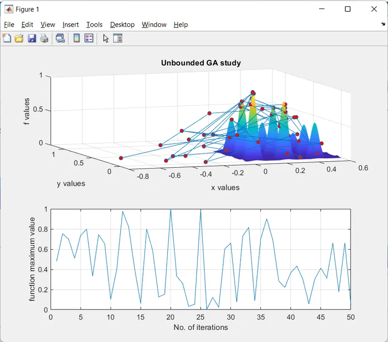
Fig 2 shown below is for case 2 we provided the boundaries for ga to run within these boundaries (0-0.4) that are lower(0) and upper(0.4) boundaries this will help us to get closer to our target maxima but still, there are some inaccuracies due to less no. of the population so that is why we will go for case 3. The function maximum value plot shows the fluctuation in ga values along the no. of iterations as we can observe that there is very minimum fluctuation in the ga values as compared to case 1.

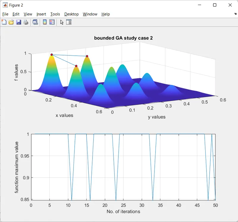
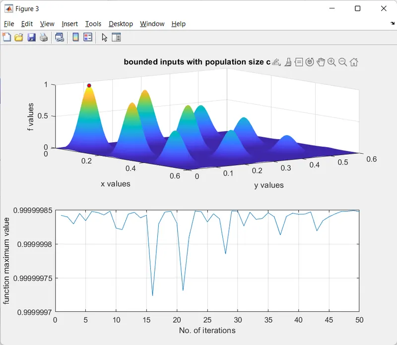
Fig 3 shown below is for case 3 this is the last case for our problem where we provided the boundaries(0-0.4) to the ga and this time we also provided a user-defined population size of 270 within the boundaries(0-0.4) of ga so this will help to achieve the exact target maxima due to the increase in the population size. The function maximum value plot shows the fluctuation in ga values along the no. of iterations as we can observe that there is a negligible amount of fluctuation which is very close to one value in the ga values as compared to cases 1 and 2.

Error faced: -

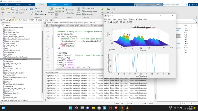
The error we faced while performing the ga study was that in 2nd case where we used the bounds there we were facing the plotting issue that is all the ga points were not visible in the plot and this is because we were not storing the ‘xopt’ and ‘yopt’ values so by default the MATLAB is plotting the last point calculated in the ga study.

Overcoming the error: -

By analyzing the code again and again we found the fault in our code and fix it by storing the values of xopt and yopt which gave us a perfect plot with all the points printed in the plot as shown in fig 2 above in the output plots.