Week 4.1 - Genetic Algorithm

Aim: To optimize the stalagmite function and find out the global maxima of the function by write a program using MATLAB and to plot for the 3 case studies and find time to take running for each case.

Objective:-

• To write a code in Matlab to optimize the stalagmite function and find the global Maxima Value of the function.
• To explain the concept of Genetic algorithm and explain the syntax of ga.
• To plot 3 case studies and for F Maxima and No. fo Iterations with respect to time.
• Plot graphs for all 3 studies and for F maximum vs no. of iterations. Title and axes labels are a must, legends could be shown if necessary.

Introduction:-

Stalagmite:

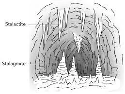
Stalagmites are upward-growing convex deposits that typically receive sustenance from an overhanging stalactite. They have tops that are flat, rounded, or somewhat hollow but lack the centre channel depicted in figure. Most importantly, the interannual fluctuation of the drip rate as well as the stalagmite's distance from the feeding stalactite's tip define the stalagmite's shape. Stalagmites that are fed by drips, on the other hand, that have an interannual consistent period between two drops produce stalagmites that resemble candles.

Function:

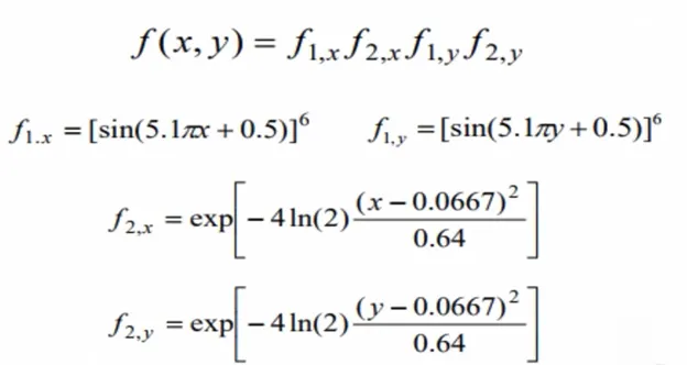
The function used in the stalagmite,

Optimization:-

Optimization is the process of making something better. We have a set of inputs and a set of outputs for every process. Finding the input values that provide the "best" output values is what this phrase alludes to. The term "best" varies depending on the issue at hand, but in mathematics, it generally refers to maximising or reducing one or more objective functions by adjusting the input parameters

The search space is the collection of every conceivable outcome or value that the inputs could have. There is a point or group of points that, when combined, provide the best solution in this search area. This point or those points in the search space are what optimization aims to locate.

Genetic Algorithm:-

The genetic algorithm, which is based on natural selection, the mechanism that propels biological evolution, is a technique for resolving both limited and unconstrained optimization issues. A population of unique solutions is repeatedly modified by the genetic algorithm. In order to create the offspring for the following generation, the genetic algorithm randomly chooses parents from the existing population at each stage. The population "evolves" toward the best option over the course of subsequent generations.

The genetic algorithm can be used to tackle a number of optimization problems, including those where the objective function is discontinuous, nondifferentiable, stochastic, or highly nonlinear and are not well suited for typical optimization algorithms. When some components of a programme must only have integer values, the evolutionary algorithm can solve these challenges.

In a genetic algorithm, there are three types of rules to reach the next generation for the current generation.

• Selection
• Crossover
• Mutation

>Selection:

Based on the fitness scaling function's scaled values, the selection function selects the parents for the subsequent generation. The expected values are what are known as the scaled fitness values. In the event that a person is chosen to be a parent more than once, more than one child will inherit that person's genes.

>Crossover:

Crossover children by selecting vector entries, or genes, from a pair of individuals in the current generation and combining them to form a child.

>Mutation:

Mutation children by applying random changes to a single individual in the current generation to create a child.

Syntax used in the Genetic Algorithm,

Here we use three syntax, that find the minimum value,

1. x=ga(fun,navrs)

This syntax used to find local unconstrained minimum value

fun- Function

navrs- No of dimensional variables

2.x=ga(fun,navrs,A,b,Aeq, beq,lb,up)

This syntax is used to find local minimum function and apply the limits by upper bounds and lower bounds,

fun-Functions

navrs- No. of dimensional variables,

A,b-linear inequalities

Aeq,beq- Nonlinear inequalities,

lb, up- upper and Lower bounds,

3. x=ga(fun,navrs,A,b,Aeq,beq,up,lb,nonlcon,intcon,options)

This syntax used in minimum function with non linear constraints by using optimoption syntax,

above syntax used to optimize the particular set of values functions collecting form the total values of arrays.

Matlab Code to optimize the stalgamite and find global maxima:

a.The programs that create a function of stalagmite,

%To create a function for stalagmite

function S=stag_fun(input_vector)

f1x=sin(5.1*pi*input_vector(1)+0.5)^6;
f1y=sin(5.1*pi*input_vector(2)+0.5)^6;
f2x=exp((-4*log(2))*((input_vector(1)-0.0667)^2/0.64));
f2y=exp((-4*log(2))*((input_vector(2)-0.0667)^2/0.64));

S=-f1x*f1y*f2x*f2y;
end

b.The Program that finding the Global Maxima,

clear all
close all
clc

%To set  input arrays of x values
x=linspace(0,0.6,150);
% To set input arrays of y values
y=linspace(0,0.6,150); 
% Create a parmaeter to run number of time in  ga
num_cases=50;


%Creating 2-Dimensional mesh
[xx,yy]=meshgrid(x,y);

%Evaluating  stalagmite function by using for loop 
for i=1:length(xx)
    for j=1:length(yy)
    input_vector(1)=xx(i,j);
    input_vector(2)=yy(i,j);
    S(i,j)=stag_fun(input_vector);
    end
end



%Study case 1-statistical behaviour
%To create a loop for upto the parameters to find optimation of max values
%using ga function wrt time taken.

tic  %To find time that while running
for k=1:num_cases
    [inputs, fopt(k)]=ga(@stag_fun,2); 
    xopt(k)=inputs(1);
    yopt(k)=inputs(2);
end
study1_time=toc;

figure(1)
subplot(2,1,1); 
hold on
surfc(xx,yy,-S);
shading interp
%plotting the optimizing values in the parameters with x, y values
plot3(xopt,yopt,-fopt,'Marker','o','markersize',5,'markerfacecolor','r');
subplot(2,1,2);
%Plotting optimized functions values
plot(fopt);
hold off
xlabel('iterations');
ylabel('Funtcion Maximum');
title('Unbounded inputs');


%Study case 2- Statistical behaviour with upper and lower bounds
%To create a loop for upto the parameters to find optimation of max values
%using ga function wrt time taken within the limits.

tic
for k=1:num_cases
    [inputs,fopt(k)]=ga(@stag_fun,2,[],[],[],[],[0;0],[1;1]);
    xopt(k)=inputs(1);
    yopt(k)=inputs(2);
end

study2_time=toc;
figure(2)
subplot(2,1,1);
hold on
surfc(x,y,-S);
shading interp;
%Plotting the optimizing values in the parameters with x, y values
plot3(xopt,yopt,-fopt,'marker','o','markersize',5,'markerfacecolor','r');
subplot(2,1,2);
%Plotting optimized functions values
plot(fopt);
hold off
xlabel('iterations');
ylabel('Funtcion Maximum');
title('Bounded inputs');


%Study case 3-Increasing GA iterations
%To create a loop for upto the parameters to find optimation of max values
%using ga function w.r.t time taken within the limits and returns set of
%parameters with options solver.

 options=optimoptions('ga');
 options=optimoptions(options,'PopulationSize',450);
tic
for k=1:num_cases
    [inputs,fopt(k)]=ga(@stag_fun,2,[],[],[],[],[0;0],[1;1],[],[],options);
    xopt(k)=inputs(1);
    yopt(k)=inputs(2);
end

study3_time=toc;
figure(3)
subplot(2,1,1);
hold on
surfc(x,y,-S);
shading interp;
%Plotting the optimizing values in the parameters with x, y values
plot3(xopt,yopt,-fopt,'marker','o','markersize',5,'markerfacecolor','r');
subplot(2,1,2);
%Plotting optimized functions values
plot(fopt);
hold off
xlabel('iterations');
ylabel('Funtcion Maximum');
title('Modifying the Population data');

Explanation:

Let's first build a random set of arrays x and y, mesh them into 2-dimensional arrays by using the mesh grid command, and then create an array called input vector with a nested loop. after using the stalagmite function formula to create a function from the stalagmite. Since the evolutionary algorithm function used to determine the Global Minima Value requires us to find the Global Maxima Value Bit, let's make the function Negative. Then, by utilising a function in the for loop command, we plot a stalagmite surface.

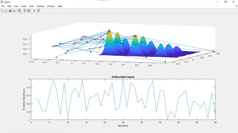
In order to determine the function minimum and the number of iterations, we must plot a graph for each of the three case studies. In the first case, we must optimise the functions that use the ga syntax up to the parameters using the tic-tac command (find time while running functions), then give the negative sign for foot because we must calculate global maxima, and finally plot the graph stalagmite with optimised values in the parameters and plot optimised functions.

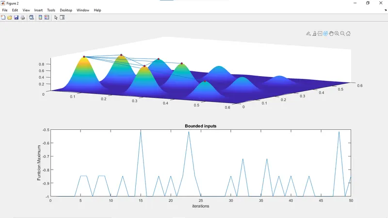
In the second case, we used ga with bounds to optimise the function, which provided greater accuracy when compared to the stalagmite's surface. In the third case, a ga syntax with solver "optimizations" and when increasing the populations to figure out the precise maxima value and plot in the stalagmite that used to be simple to locate were used to determine the global maxima value of the array.

>Graphs:

Stalagmite Graph:

Plot for unbounded values

The plot of Bounded Inputs,

The plot using Increase the Populations,

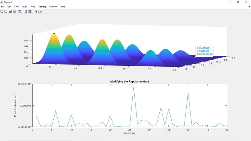
The above plot has obtained the Global maxima as per the objective

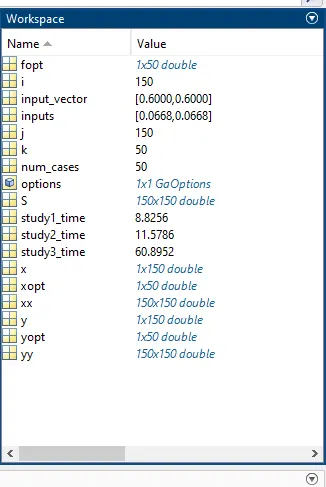
Workspace data:

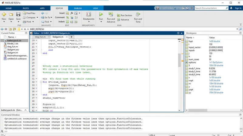
MATLAB script page,

Conclusion:

After optimising the Stalagmite function, we discovered that the Global Maxima value is (x=0.0668,y=0.0668). A brief explanation of the Genetic algorithm and the ga syntax used in the application have been provided. Plotting the three case studies that were used to determine the global maxima revealed that they all had the same values when repeated several times.