Week 3 - Solving second order ODEs

1. The program in Matlab that will simulate the pendulum motion with respect to the inputs given in between 0-20 sec, for angular displacement=0,angular velocity=3 rad/sec at time t=0 is as follows:-

The video link for the simulation of the motion of the pendulum is : https://youtu.be/aS20tNp3XAg

The program for simulating the simple pendulum motion is as follows:-

% Program to solve and create animation for a motion of Simple Pendulum

clear all
close all
clc

%The various inputs for simple pendulum motion i.e damping co-efficient b
%in kg/s, gravitational acceleration g in ms^-2, Length l in m and Mass m is kg.  

b=0.05;

g= 9.81;

l= 1;

m = 1;


% Initial condition of angular motion theta will be in array form having
% initial displacement and initial velocity at the start of the motion i.e
% taking initial angular displacement as 0 and initial angular velocity as
% 3 rad/s

theta_0 = [0;3];

% Now giving time array for the timespan t in seconds

t_span = linspace(0,20,500)

% Calling ODE solver and calling the function defined for motion of simple pendulum
% Here ode45() is used where independent value time and dependent value
% theta are given as inputs, then calling defined function ode_solver()
% approximating the motion of pendulum from the pendulum equation with
% damper, themn giving the limits for the independent variable of time and
% initial conditions of the pendulum containing initial dispalcement and
% velocity at t=0 which will give us the output which will be stored in
% output t array and displacement and velocity will be stored in the output
% array with respect to t.

[t,output] = ode45(@(t,theta) ode_solver(t, theta, b, g, l, m),t_span, theta_0);




%As we got the different angular displacement values between 0-20 seconds
%stores in output_result array but it is in the form of radians . Need to
%convert the polar co-ordinates to angular co-ordinates. Hence we can
%covert to cartesian co-ordinates using sine and cosine plot. 
% After converting the co-ordinates into cartesian form in the for loop for
% each iteration plotting the movement of pendulum with respect to time
% from the diplacement value stored in the output vector




for i= 1:length(output)

     figure(1)

       x1 = l*sin(output(i,1))
    
       y1 = -l*cos(output(i,1))

       x0 = 0
       y0 = 0

     
%Plotting the horizontal line for the object on which the string tied end begins which we considered as origin.
     
       plot([-2 2], [0 0], 'linewidth',2 )
% using hold on command to retains all the plots in the same figure(1)
     
       hold on
      
% Plotting the pendulum and the various co-ordinates it will have  with
% respect to time
      plot([x0 x1],[y0 y1],'linewidth',3,'color','r')

% Plotting the string and the sphere of mass present at the free end of the pendulum    
      
      plot(x1 ,y1 ,'Marker','o','MarkerSize',15 ,'MarkerFaceColor','g')
      
      axis([-2 2 -2 2])
      
% Giving hold off command here that will remove the trace of other figures with different 
% dispalcement value and time , if not multiple figures at different iterations will be left in the
% animation
     
      hold off

      %A variable M(i) is defined to capture the frames of plot of all
      % iterations of the for loop 

      M(i) = getframe(gcf);

      % the for loop will end once i reaches the last iteration 
     
end


%Program to animate the movement of simple pendulum by using the figures
%captured in the M array 


movie(M)
videofile = VideoWriter("Simple_Pendulum.avi", 'Uncompressed AVI')
open(videofile)
writeVideo(videofile,M)
close(videofile)

1. The above program gives us the simulation of the motion of simple pendulum with a damper.
Here, we use clear all to clear the workspace window, close all to close all the figures if are open and clc to clear the command window.

2. Then we defined the variables for inputs provided in the question to intergrate in the equation of simple pendulum motion to achieve the angulat displacement and velocity with respect to time . the various inputs are
g = gravity in m/s2,
L = length of the pendulum in m,
m = mass of the ball in kg,
b=damping coefficient.

3. Then time limits are given i.e between 0 and 20 seconds for which we defined a variable t_span and gave 500 iterations between the time limits and then initial conditions of the motion for pendulum i.e angular displacement and angular velocity is provided at time t= 0 which we clubbed together in a variable theta_0 as coloumn matrix.

4. Then we use the ode45() function to solve the pendulum equation which can be used to solve first order differential equations where we define the independent and dependent quantity after @ and then we call the function ode_solver(t, theta, b, g, l, m) from another program with the same name in which we have broke down the 2nd order differential of the pendulum into first order differential equation after which we provide the time limits i.e the array t_span and the initial condition of the pendulum. The ODE45 solver then approximates the value of angular displacement and angular velocioty with respect to to each instance in the time array aand the output is stored in an array of time and output where the output array stores the angular displacement in the first column and angular displacement in the second. We then proceed to animate the motion of the pendulum with the achieved output array.

5. We start the for loop to collect the co-ordinates of the pendulum with respect to the time interval for each instance between the time limit 0 to 20 seconds. The counter i is provided with the range of the length of the output matrix using range operator and length() fuction which takes the no of longest values present from the row matrix i.e 500 . So the for loop should run for 500 times before coming to a stop. In the for loop we covert the the value of angular displacement from polar co-ordinates to cartesian co-ordinates to plot the various diplacement co-ordinates with respect to each time iteration i.e defining it in sine an cosine forms and not using cosd or sind as the value is in radians hence using cos() and sin() functions and storing the angular displacement in x1 and y1 array and defining the co-ordinates x0 and y0 as (0,0) along which the string will swing . the value of y is given negative sign as we are plotting the displacements along negative y axis.

6. After this we give the plot command making a horizontal line along the x axis alon which the string will hang at the origin . We then give "hold on" command to retains all the plots in the single figure otherwise the plot command will give the output of the last plot command given. We then plot the x1 and y1 values with respect to t using plot() giving it color and linewidth properties. After this we give one more plot command to plot a sphere at the free end of the string that will represent the mass m of the pendulum using marker() function as gicing additional marker properties such as size and facecolor for the sphere. We then using axis() define the axis of x and y axis accordingly so that output can be visible

7. We then use "hold off" command so that it will remove the plot of previous time iterations of the pendulum otherwise resulting in multiple images of the string at different time and displacement values .

8. We then define an array M storing figures at each iterations i.e at different displacement at different time intervals which we will use to create the animation.

9. Lastly we write the code for creating a short animation video by catenation of all the frames stores in variable M using movie() command which runs the movie M times and thenwe go ahead create a variable videofile which stores the video created using Videowriter(a,b) command where a is the name of the file and b is the format of the video file and then we use open() fn to open the created videofile and use writeVideo() fn to writes data from an array to the video file associated with videofile and M signifies the figures and this should be used after open(0 fn otherwise it will throw an error and finally we use close() to close the video once played.

b. The program to define the function after simlifying the pendulum motions equation in first order differential equation is as follows:-

%Creating function for simple pendulum motion in first order ode by
%assuming angular velocity as theta2 and angular displacement as theta1

function [dtheta_dt] = ode_solver(t, theta, b, g, l, m)
        
% Defining theta1 and theta2 in terms of theta otherwise will gett error of
% undefined variables for theta 1 and theta 2
       
        theta1 = theta(1)
        theta2 = theta(2)

% Forming two equation and simplying the 2nd order ode in first order and returning value of theta 1 and theta 2 i.e nothing
% but angular displacement and angular velocity stored in array dtheta_dt and storing it as coloumn
% matrix so that the function works with respect to t 
        
         dtheta1_dt = theta2 ;

      dtheta2_dt = -(b/m)*theta2 - (g/l)*sin(theta1);

      dtheta_dt = [dtheta1_dt; dtheta2_dt];

end     

We wrote this code to define a function ode_solver(t, theta, b, g, l, m) that will define the equation of the pendulum in first order differential equation. here we have simplified the second order differential equation of the pendulum in the first order differential equation in form of theta1 and theta2 respectively where theta1 stores the value of angular dislacement and theta2 for angular velocity . Then storing them both in a array in dtheta_dt as coloumn matrix which acts as output array

This simplied function representing the motion of pendulum is then called in the main program in ode45() solver to get the angular dispalcement and velocity . The file name is the same as function name so that it can be called in the main program with the name and giving the inputs accordingly as defined in the function.

After defining the function we close it with end command .

c. The output is as follows:-

The video link showing the simulation is already provided above .

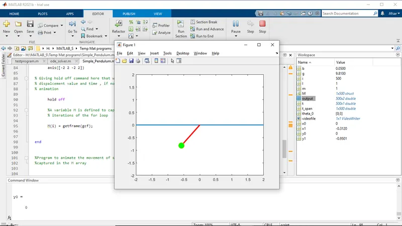
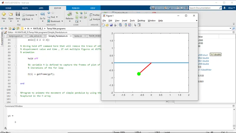
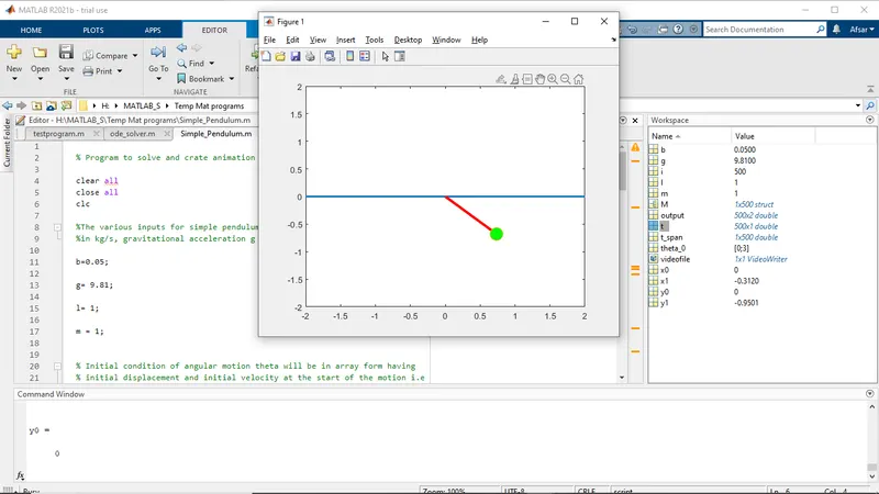
Hence the motion of the pendulum between 0-20 sec, for angular displacement=0,angular velocity=3 rad/sec at time t=0 is simulated .