Week 4.1 - Genetic Algorithm
OBJECTIVE :
To optimise the stalagmite function and find the global maxima of the function by using MATLAB.
Genetic Algorithm :
Genetic Algorithm (GA) is a branch of field of study called evolutionary comutation. It is based on evolution theory by Darwin. GA is used to optimize a given function to find its maximum or minimum value. The basic components of a GA are
1. Fitness function : It is the function that GA is trying to optimize.
2. A population of chromosome : It is the numerical values that represent all the solutions to the function. The selection operator chooses some of the chromosomes (with replacement) for reproduction based on probability distribution. fitter the chromosome more likely it is to be selected.
3. Cross over : This operator swaps in random a subsequence of two of the chosen chromosomes to create two offspring. Usually each chromosome is converted into binary code and then cross over is done from one parent chromosome into another.
4. Mutation : Mutation operator randomly flips individual bits in the new chromosomes.
Advantages of Genetic Algorithms:
1) They usually perform better than traditional feature selection techniques.
2) Genetic algorithms can manage data sets with many features.
3) They don't need specific knowledge about the problem under study.
4) These algorithms can be easily paralelized in computer clusters.
Working of Genetic Algorithm:
1) The algorithm begins by creating a random initial population.The algorithm then creates a sequence of new populations.
2) At each step, the algorithm uses the individuals in the current generation to create the next population.
To create the new population, the algorithm performs the following steps:
a) Scores each member of the current population by computing its fitness value. These values are called the raw fitness scores.
b) Scales the raw fitness scores to convert them into a more usable range of values. These scaled values are called expectation values.
c) Selects members, called parents, based on their expectation.
d) Some of the individuals in the current population that have lower fitness are chosen as elite. These elite individuals are passed to the next population.
e) Produces children from the parents. Children are produced either by making random changes to a single parent—mutation or by combining the vector entries of a pair of parents—crossover.
e) Replaces the current population with the children to form the next generation.The algorithm stops when one of the stopping criteria is met.
Function Code
function [f] = stalagmite(input)
x = input(1);
y = input(2);
f1x = (sin(5.1*pi*x + 0.5))^6;
f1y = (sin(5.1*pi*y + 0.5))^6;
f2x = exp((-2.7726)*(x-(0.0667))^2/0.64);
f2y = exp((-2.7726)*(y-(0.0667))^2/0.64);
f = -(f1x*f1y*f2x*f2y);
endMain Code:
clear all
close all
clc

%Defining our search space
x = linspace(0,0.6,150);
y = linspace(0,0.6,150);
[xx,yy] = meshgrid(x,y);
num_cases = 80 ;

%calling stalagmite function
for i = 1:length(xx)
    for j = 1:length(yy)
        input_vector(1) = xx(i,j);
        input_vector(2) = yy(i,j);
        f(i,j) = stalagmite(input_vector);
    end
end

%Study 1 - Statistical behavior
tic
for i=1:num_cases
    [inputs, fopt(i)] = ga(@stalagmite,2);
    xopt(i) = inputs(1);
   yopt(i) = inputs(2);

end

study1_time = toc

figure(1)
subplot(2,1,1)
hold on
surfc(xx,yy,f)
shading interp
title('Unbound inputs')
xlabel('X values')
ylabel('Y values')
plot3(xopt,yopt,fopt,'marker','o','markersize',5,'markerfacecolor','r')

subplot(2,1,2)
plot(fopt)
xlabel('Iterations')
ylabel('Function maximum')

%Study 2 - Statistical behavior with upper and lower bounds
tic
for i=1:num_cases
    [inputs, fopt(i)] = ga(@stalagmite,2,[],[],[],[],[0;0],[0.6;0.6]);
    xopt(i) = inputs(1);
   yopt(i) = inputs(2);
end

 study2_time = toc

figure(2)
subplot(2,1,1)
hold on
surfc(xx,yy,f)
shading interp
title('Bounded inputs')
xlabel('X values')
ylabel('Y values')
plot3(xopt,yopt,fopt,'marker','o','markersize',5,'markerfacecolor','r')
subplot(2,1,2)
plot(fopt)
xlabel('Iterations')
ylabel('Function maximum')

%Study 3 - Increasing GA iterations
options = optimoptions('ga')
options = optimoptions(options,'populationSize',200)

tic
for i=1:num_cases
    [inputs, fopt(i)] = ga(@stalagmite,2,[],[],[],[],[0;0],[0.6;0.6],[],[],options);
    xopt(i) = inputs(1);
   yopt(i) = inputs(2);
end

 study3_time = toc

figure(3)
subplot(2,1,1)
hold on
surfc(xx,yy,f)
shading interp
xlabel('X values')
ylabel('Y values')
plot3(xopt,yopt,fopt,'marker','o','markersize',5,'markerfacecolor','r')
subplot(2,1,2)
plot(fopt)
xlabel('Iterations')
ylabel('Function maximum')
STUDY 1:
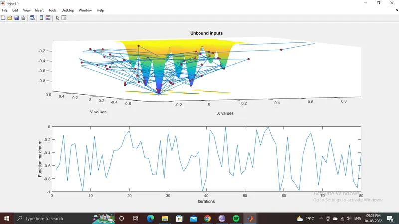
there are no lower and upper limits hence the GA does not the search space is between 0 and 1.
Hence each time the program is executed different optimum values are are obtained as shown in the plot 2.
STUDY 2:
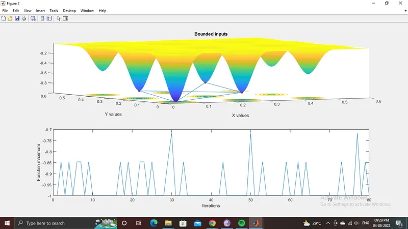
most of the maximum values obtained in each iteration varies between (-1) and (-0.7).
This method narrows down the maximum values to 4 points as shown in the plot 1.
STUDY 3:
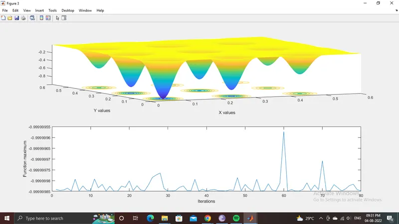
In the 3rd study the global maximum obtained is accurate and is narrowed down to a value of -0.999999 as shown in the graphs.
CONCLUSION :
Optimised stagalmite function and global maxima of function is found successfully by using MATLAB.
References
https://in.mathworks.com/help/gads/how-the-genetic-algorithm-works.html?s_tid=mwa_osa_a
https://mech.iitm.ac.in/nspch52.pdf
https://www.tutorialspoint.com/genetic_algorithms/genetic_algorithms_introduction.htm