Week 4.1 - Genetic Algorithm
Aim-By using the ‘ga’ find the global maxima.
Theory-
Ga is an inbuilt command in matlab used for optimisation problem in designing of airplane here we are calculating the drag force by using ga command we can find the optimum values of drag force. It also can be used for manufacturing process.
In the genetic algorithm there are 3 main rule-
Selection rule select the individuals to form parents
Crossover rule combine the two parent to form child.
Mutation rule select the best from parent and child and keep best of them and form parent and child.
‘syntax for ga’
x = ga(fun,nvars,A,b,Aeq,beq,lb,ub)
x = ga(fun,nvars,A,b,Aeq,beq,lb,ub,nonlcon)
x = ga(fun,nvars,A,b,Aeq,beq,lb,ub,nonlcon,options)
x = ga(fun,nvars,A,b,Aeq,beq,lb,ub,nonlcon,intcon)
x = ga(fun,nvars,A,b,Aeq,beq,lb,ub,nonlcon,intcon,options)
[x,fval,exitflag,output] = ga(___)
[x,fval,exitflag,output,population,scores] = ga(___)
Programme-
clear all
close all
clc
%defining our search space
x=linspace(0,0.6,100);
y=linspace(0,0.6,100);
%creating 2 dimensional array
[xx,yy]=meshgrid(x,y)
%evaluating the stagalmite function
for i=1:length(xx);
for j=1:length(yy);
input_vector(1)=xx(i,j);
input_vector(2)=yy(i,j);
f(i,j)=stalagmite_func(input_vector);
end
end
surf(xx,yy,f)
xlabel('x value')
ylabel('y value')
shading interp
[inputs,fval]=ga(@stalagmite_func,2)
Above shows the main programme.
function [stalagmite]=stalagmite_func(input_vector)
x=input_vector(1)
y=input_vector(2)
f1_x=(sin(5.1*pi*x+0.5)).^6;
f2_y=(sin(5.1*pi*y+0.5)).^6;
f3_x=exp((-4*0.6931).*(x-0.0667)^2/(0.64))
f4_y=exp((-4*0.6993).*(y-0.0667)^2/(0.64))
stalagmite=(f1_x.*f2_y.*f3_x.*f4_y)
end
Above shows the function command programme.
Programme explanation-
Clear all, close all, clc used for deleting the previous page.
We are taking one dimensional array by using the linspace command and after that we are creating two dimensional array by using meshgrid command.
Forloop command is used to get the repeating the values coming from stagalmite function.
Surf is used for showing the function
Shading interp is used for shading the peaks and valley by removing the grid lines.
Ga is an inbuilt command in matlab shows optimum values and used for minimize the value for obtaining the global maxima we are giving negative sign for equation in function command.
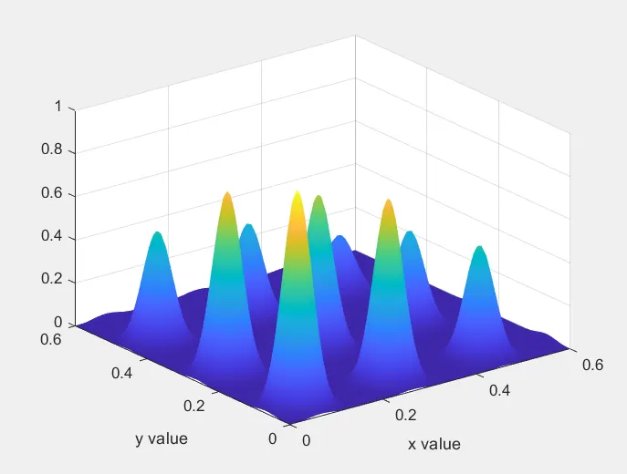
For global maxima there are 3 study which are below-
To obtain global maxima we are giving negative for the equation in function command.
Study[1] programme-
x = linspace(0,0.6,150);
y = linspace(0,0.6,150);
num_cases = 50;
%creating 2 dimensional array
[xx,yy] = meshgrid(x,y);
% evaluating the stalagmite function
for i = 1:length(xx)
for j = 1:length(yy)
input_vector(1)= xx(i,j);
input_vector(2)= yy(i,j);
f(i,j) = stalagmite_funcc(input_vector);
end
end
%study_1 statistical behaviour
tic
for i = 1:num_cases
[inputs,Fopt(i)] = ga(@stalagmite_funcc,2);
xopt(i) = inputs(1);
yopt(i) = inputs(2);
end
study_time_1 = toc;
%plotting
figure(1)
subplot(2,1,1);
hold on
surfc(xx,yy,f);
shading interp;
ylabel('Y data');
xlabel('X data');
plot3(xopt,yopt,Fopt,'marker','o','markersize',7,'markerfacecolor','r')
title('Unbounded Inputs')
subplot(2,1,2)
plot(Fopt)
xlabel('Iterations')
ylabel('Maximum function')
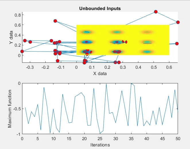
tic toc is used for time period this shows the optimum values.
Study[2]-
%study_2 statistical behaviour
tic
for i = 1:num_cases
[inputs,Fopt(i)] = ga(@stalagmite_funcc,2,[],[],[],[],[0;0],[1;1]);
xopt(i) = inputs(1);
yopt(i) = inputs(2);
end
study_time_2 = toc;
%plotting
figure(2)
subplot(2,1,1);
hold on
surfc(xx,yy,f);
shading interp;
ylabel('Y data');
xlabel('X data');
plot3(xopt,yopt,Fopt,'marker','o','markersize',7,'markerfacecolor','r')
title('bounded Inputs')
subplot(2,1,2)
plot(Fopt)
xlabel('Iterations')
ylabel('Maximum function')
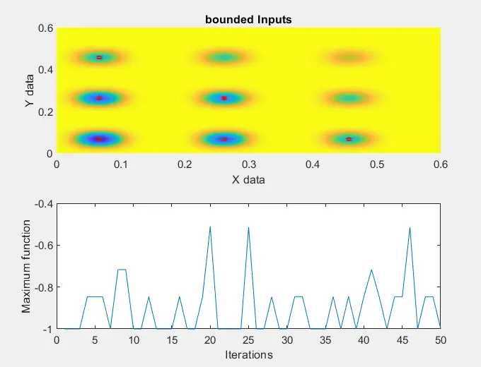
this shows the optimum values than study 1.
Study[3]
%study_3 bounding with increasing population size
options=optimoptions('ga');
options=optimoptions(options,'populationsize',150);
tic
for i = 1:num_cases
[inputs,Fopt(i)] = ga(@stalagmite_funcc,2,[],[],[],[],[0;0],[1;1],[],[],options);
xopt(i) = inputs(1);
yopt(i) = inputs(2);
end
study_time_3 = toc;
%plotting
figure(3)
subplot(2,1,1);
hold on
surfc(xx,yy,f);
shading interp;
ylabel('Y data');
xlabel('X data');
plot3(xopt,yopt,Fopt,'marker','o','markersize',7,'markerfacecolor','r')
title('bounding with increasing population size')
subplot(2,1,2)
plot(Fopt)
xlabel('Iterations')
ylabel('Maximum function')
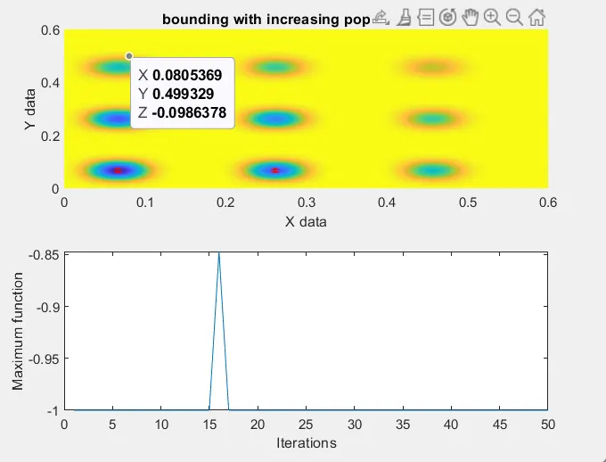
this show the optimum values better than the study 1 and study 2 but it will take more than study 1 and study 2.