Week 3 - Solving second order ODEs

Programme report on ODE-

Aim-By using the ode command solving the 2^nd order differential equations.

Governing equations-

d^2theta/dt^2+(b/m)dtheta/dt+(g/l)sin theta=theta

b=damping

m=mass

g=gravity

l=length

Objective- By using the ode command solve the above differential equation and also using function in MATLAB.

Programme explanation-

b=0.05 (b is damping coefficient)

g=9.81 (g is gravitational force)

l=1 (l is length of pendulum)

m=1 (mass of the pendulum)

by using the above values

%initial condition

theta_0=[0;3];

-0 shows the displacement and 5 shows the velocity.

%time points

t_span=linspace(0,20,500);

-t_span shows the time period of pendulum 0 to 20 sec and 500 values from them.

%solve ode

[t,results]=ode45(@(t,theta)ode_func(t,theta,b,g,l,m),t_span,theta_0);

-t,results=Solution vectors; matlab returns results for each time ‘t’.

ode45=Integral command in matlab.

Ode_func=Function that returns dy =f(t,y)

t,theta,b,g,l,m =Defined in starting i.e input condition.

t_span=shows the time period

theta_0=Shows the displacement and velocity.

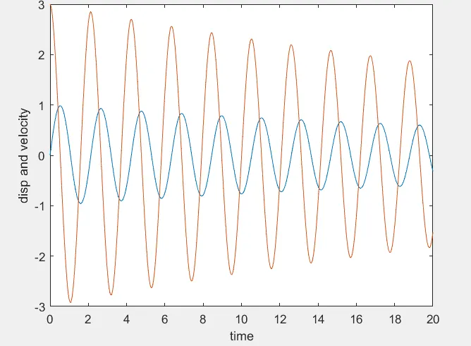
plot(t,results(:,1))

-by using the plot command plotting the values that we obtained in command window it shows the 1 column vector.

hold on

plot(t,results(:,2))

-by using this shows the second column.

ylabel('Plot')

-by using this we are labelling to y-axis as plot.

xlabel('time')

-by using this we are labelling to x-axis as time.

We are using the forloop command for animation of pendulum because pendulum position repeats.

%creating animation

for i=1:length(results(:,2)) (i repeating the result and 2 shows the 2^nd column)

figure(2)

x1=l*sin(results(i,1)); (x1 and y1 we are calculating the position of pendulum by using trignometry)

y1=-(l*cos(results(i,1)));

plot([-1.5 1.5],[0 0],'linewidth',3,'color',[0.54 0.42 0.52])

axis([-1 1 -1.5 1])

hold on

line([x0 x1],[y0 y1],'linewidth',5,'color','g'); (showing the position of pendulum)

plot(x1,y1,'o','markersize',15,'markerfacecolor','r'); (It shows the ball attached to pendulum i.e ‘o’ and size of the ball)

hold off

M(ct)=getframe(gcf); (It is used for storing the image)

ct=ct+1;

end

%create movie

movie(M);

videofile=VideoWriter('SimplePendulum_oscillation.avi','Uncompressed AVI'); (It is showing the the empty folder for video file)

open(videofile);

writeVideo(videofile,M);

close(videofile);

As we mention above we need to define the ode_func then go to another new file and define the deferential equations as below- The function commands means files that take certain inputs, executes sequence of steps and returns output at the end.

function[dtheta_dt]=ode_func(t,theta,b,g,l,m)

-dtheta_dt=output

Ode_func(t,theta,b,g,l,m)=inputs.

theta1=theta(1)

theta2=theta(2)

dtheta1_dt=theta2;

dtheta2_dt=-(b/m)*theta2-(g/l)*sin(theta1);

dtheta_dt=[dtheta1_dt;dtheta2_dt];

end

As mentioned in the governing equation we define that equation in the function command.

Output results-

below graph shows the graph disp.and velocity vs time.