Week 4.1 - Genetic Algorithm

% Aim-To calculate the maxima of the given function

%Objective-

1.) write a matlab program to evaluate the maxima for the given function

2.) Study the geometric algorithm

% Explanation GA

Geometric algorithm-it is a optimization technic based on genetic and natural selection principle

it predicts the trend in population size

GA produces a population of points at each iteration,the best point in the population approches an optimal solution.

Dureing optimization the Ga follows the below order

1.Selection

2.Cross over

3.Mutation

Selection is based on concept of random selection as per the fitness score from the population size , thus allows them to pass there genes to the next generation

Cross over- this refers to the mateing between individuals.two individuals are selected and cross over are changed thus

creating a completly new individual.

Mutation operator-insert a random genie into the new individual to avoid premature convergence.

Process for GA is summerize roughly as below
1) Randomly initialize populations 
2) Determine fitness of population
3) Until convergence repeat:
      a) Select parents from population
      b) Crossover and generate new population
      c) Perform mutation on new population
      d) Calculate fitness for new population

-Stopping criteria
when we get a maximum sigular value for the iteration that satisfy the function we need not to go further itrations. here we can stop
 

-Syntax for Ga

% Matlab code for maximizing the function

close all 
clear all 
% use of stalagmite
% function for finding  out maxima 
x=linspace(0,0.6,150); % create a one dimeshinal array
y=linspace(0,0.6,150);
num_case=150; % number of values 150

%creating the 2 Dimensional mesh
[xx,yy]= meshgrid(x,y);   % creating a 2 D array of matrix , use closed brackets

% Evaluating stalagmite function 
for i=1:length(xx)  % for loop starting from interval 1 till last value of xx
    for j=1:length(yy)   % for loop starting from interval 1 till last value of yy
        input_vector(1)=xx(i,j); % assining a new variable to store matrix value of xx 
        input_vector(2)=yy(i,j);% assining a new variable to store matrix value of yy

        f(i,j) = stalagmite_f(input_vector);%ncalls the staligmite_f function

    end
end

surfc (x,y,f) % creates the surface plot 
shading interp % colours  

% 1st case
tic   % Command used to start timer

 for i=1:num_case  %for loop starts with interval 1 for all values of num_case
     [inputs,fopt(i)]=ga(@stalagmite_f,2);
     xopt(i)=inputs(1);
     yopt(i)= inputs(2);
 end
 fopt = -fopt
 f = -f
 Study1time = toc
 figure(1)
 subplot(2 ,1, 1) % create a plot inside a plot with no of rows ,colums and position
 hold on
 surfc(x,y,f) % function to create a surface plot
 shading interp
 plot3(xopt,yopt,fopt,'color','b','marker','o','markersize',5,'MarkerFaceColor','r')
 title('Unbounded inputs');
 subplot(2, 1, 2)
 plot(fopt,'color','b','linewidth',1)
 xlabel('itrations')
 ylabel('function minimum')

 % 2nd case Optimization with bounded inputs.
 tic
 for i=1:num_case
 [input,fopt2(i)]= ga(@stalagmite_f,2,[],[],[],[],[0;0],[0.6;0.6]);% stalagmite function for bounded inputs for linearity of equations
 xopt(i)=input(1);
 yopt(i)=input(2);
 end
 fopt2=-fopt2
   f = -f

 study2time=toc;
 figure(2)
 subplot(2,1,1);
 hold on
 surfc (x,y,f);
 shading interp
 title('bounded inputs')
 plot3(xopt,yopt,fopt2,'color','b','marker','o','markersize',5,'MarkerFaceColor','r')

 title('bounded inputs')
  subplot(2,1,2);
 plot(fopt2,'color','b','linewidth',1)
 xlabel('itrations')
 ylabel('limits ')


 %Study 3 Increasing the population size.
 options=optimoptions('ga');
 options=optimoptions(options,'populationsize',200);
 tic
  for i=1:num_case
 [input,fopt3(i)] = ga(@stalagmite_f,2,[],[],[],[],[0; 0],[0.6; 0.6],[],[],options);
xopt(i)=input(1);
yopt(i)=input(2);
  end
  fopt3=-fopt3
  f = -f
 study2time=toc;
 figure(3)
 subplot(2,1,1);
 hold on
 surfc (x,y,f);
 shading interp
 title('bounded inputs')
 subplot(2,1,2);
 plot3(xopt,yopt,fopt3,'color','b','marker','o','markersize',5,'MarkerFaceColor','r');
 title('bounded inputs')
 plot(fopt3,'color','b','linewidth',1)
 xlabel('itrations')

 
%Function Program

function[f_max]=stalagmite_f(input_vector)

x = input_vector(1);
y = input_vector(2);
fx=(sin(5.1*pi*x+0.5))^6;
fy=(sin(5.1*pi*y+0.5))^6;
fxx=exp((-4*log(2)*(x-0.0667)^2)/(0.64));
fyy=exp((-4*log(2)*(y-0.0667)^2)/(0.64));
f_max=-(fx*fy*fxx*fyy);
end

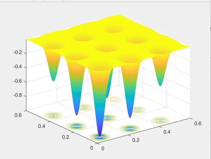
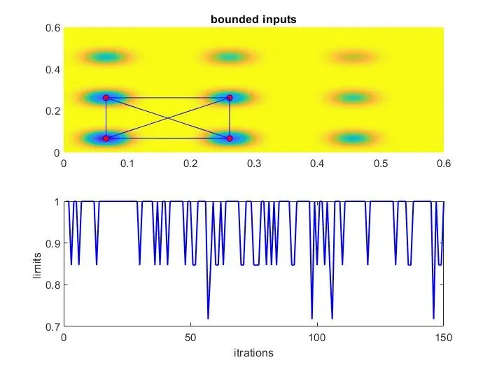
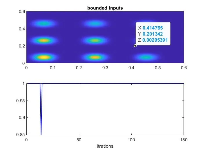
% Outcome of the above program

1.

case 2.

case-3

% Errors while codeing

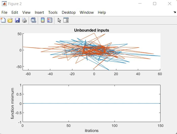
It is caused due to skipping of plot () after subplot (2,2,1). correction done by commanding plot() after sunb plot.

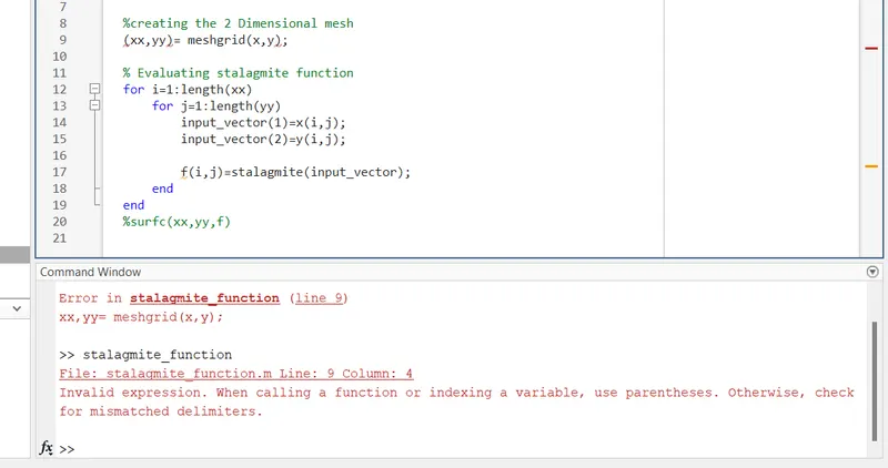
In line no .9 -() brackets used instead of [] .by useing mesh grid command we are combining the x and y arrays to form a 2D matrix thus [] are used to determine array.

this error corrected by changing the brackets paranthesis.

% Conclusion

Thus we studied the optimization useing ganetic algorithm technic

Written a program to find out maxima for the given function.