Project 2 - Rankine cycle Simulator
Aim-To study the Rankine Cycle by programming it in matlab .
Objective-
1)Script the rankine cycle simulator
2) Evaluate the state points
3) plot the results
Theory-
The Rankine cycle is a model used to predict the performance of steam turbine systems. It was also used to study the performance of reciprocating steam engines. The Rankine cycle is an idealized thermodynamic cycle of a heat engine that converts heat into mechanical work while undergoing phase change. It is an idealized cycle in which friction losses in each of the four components are neglected. The heat is supplied externally to a closed loop, which usually uses water as the working fluid.
The Rankine cycle closely describes the process by which steam-operated heat engines commonly found in thermal power generation plants generate power. Power depends on the temperature difference between a heat source and a cold source. The higher the difference, the more mechanical power can be efficiently extracted out of heat energy, as per Carnot's theorem. The heat sources used in these power plants are usually nuclear fission or the combustion of fossil fuels such as coal, natural gas, and oil, or concentrated solar power. The higher the temperature, the better.
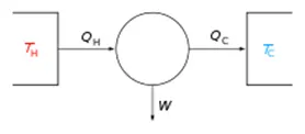
Figure 1. Classical Carnot Heat Engine
The efficiency of the Rankine cycle is limited by the high heat of vaporization of the working fluid. Also, unless the pressure and temperature reach super critical levels in the steam boiler, the temperature range the cycle can operate over is quite small: steam turbine entry temperatures are typically around 565 °C and steam condenser temperatures are around 30 °C. This gives a theoretical maximum Carnot efficiency for the steam turbine alone of about 63.8% compared with an actual overall thermal efficiency of up to 42% for a modern coal-fired power station. This low steam turbine entry temperature (compared to a gas turbine) is why the Rankine (steam) cycle is often used as a bottoming cycle to recover otherwise rejected heat in combined-cycle gas turbine power stations.
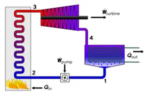
Figure 2. Rankine Cycle Layout [1 – Pump, 2 – Boiler, 3 – Turbine, 4 – Compressor]
The cold source (the colder the better) used in these power plants are usually cooling towers and a large water body (river or sea). The efficiency of the Rankine cycle is limited on the cold side by the lower practical temperature of the working fluid. The working fluid in a Rankine cycle follows a closed loop and is reused constantly. The water vapor with condensed droplets often seen billowing from power stations is created by the cooling systems (not directly from the closed-loop Rankine power cycle). This 'exhaust' heat is represented by the "Qout" flowing out of the lower side of the cycle shown in the T–s diagram below. Cooling towers operate as large heat exchangers by absorbing the latent heat of vaporization of the working fluid and simultaneously evaporating cooling water to the atmosphere.
While many substances could be used as the working fluid in the Rankine cycle, water is usually the fluid of choice due to its favorable properties, such as its non-toxic and unreactive chemistry, abundance, and low cost, as well as its thermodynamic properties. By condensing the working steam vapor to a liquid the pressure at the turbine outlet is lowered and the energy required by the feed pump consumes only 1% to 3% of the turbine output power and these factors contribute to a higher efficiency for the cycle. The benefit of this is offset by the low temperatures of steam admitted to the turbine(s). Gas turbines, for instance, have turbine entry temperatures approaching 1500 °C. However, the thermal efficiency of actual large steam power stations and large modern gas turbine stations are similar.
%% Program script for rankine cycle

clear
close
clc
% Program script to find out Net work output and back work ratio for
% Rankine cycle
%Inputs
% finding out the work efficiency and back work ratio for Rankine cycle
%users inputs
fprintf('program to evaluate the Rankine cycle used in boiler \n')
fprintf('Process (1-2)-Isentropic Expansion in Turbine \n')
fprintf('Process (2-3)-Isobaric heat rejection to the conndensor \n')
fprintf('Process (3-4)-Isentropic Compression in Compressor \n')
fprintf('Process (4-1)- Heat addition in boiler \n')

T1=400;% input temp in kelvin
P1=30;% input Pressure to turbine inlet in bar
P2=0.05; %output pressure at turbine outlet
% calculateing the state points
% point 1

s1 = XSteam('s_pt',30,400); %specific entropy at point 1
h1 = XSteam('h_pt',30,400);% specific enthalpy at point 1

% point 2
sf2=XSteam('sL_p',P2);%specific entropy of fluid at point 2
sg2=XSteam('sv_p',P2);%specific entropy of gas at point 2
hf2=XSteam('hl_p',P2);% specific enthalpy of fluid  at point 2
hg2=XSteam('hv_p',P2);% specific enthalpy of gas at point 2
s2 = s1;
X2=((s2-sf2)/(sg2-sf2)); %dryness factor at point 2
h2=hf2+(X2*(hg2-hf2));% Specific ent5halphy at point 2
Tsat2=XSteam('Tsat_p',P2);% Saturation temp. at point 2
Cp2=XSteam('CpV_p',P2);% specific heat at point 2

Wf=h1+h2;
Wt=h1-h2;%wprk done by turbine

% At point 3
hf3=XSteam('hL_p',P2);%enthalphy  of fluid at point 3
sf3=XSteam('SL_p',P2);%specific entropy of fluid at point 3
h3=hf3;
v3=XSteam('vL_p',P2);

%for point 4
hf4=XSteam('hL_p',P1);%specific enthalphy of fluid at point 4
sf4=XSteam('SL_p',P1);%specific entropy of fluid at point 4
P4=P1;
P3=P2;
wp=v3*(P4-P3)*100;% Pump work done
h4=h3-wp;% Specific enthalphy at point 1
Wnet=Wt-wp;% Net work done

%heat added to the process Qin
Qin=h1-h4;

% heat rejection from the process

Qout=h2-h3;

%Thermal efficiency of rankine cycle
Thermal_effi=(Wnet/Qin)*100;

%Specific steam consumption=(mass flow ret/net work done)

SSC=3600/Wnet;

% calculation of Temperatures, heat capacity
T3 = XSteam ('Tsat_p',P3);	  % Saturation Temperature at Pressure 3
s3=XSteam('sL_p',P3);

T2 =  T3;                     % Becuase of Constant Pressure Heat addition
s4=s3;
P4=P1;
Cp4 = XSteam('Cp_ps',P4,s4);  % Specific isobaric heat capacity
Cv4 = XSteam('Cv_ps',P4,s4);  % Specific isochoric heat capacity
k =  Cp4/Cv4;                 % Adiabatic index
T4 = T3/((P3/P4)^((k-1)/k));  % Temperature at State point 4

%  Calcula tion  of  Other  constant  for saturated  liquid  and  Vapour
T6=XSteam ('Tsat_p', P1) ;	%  Saturated  Temperature at Pressure 1
s5=XSteam ('sL_p', P1) ;	    %  Saturated  Liquid  entropy  at pressure 1
s6=XSteam ('sV_p', P1) ;	    %  Saturated  Vapour  entropy  at Pressure  1
h5=XSteam ('hL_p', P1) ;	    %  Saturated  Liquid  Enthalpy  at Pressure  1
h6=XSteam ('hV_p', P1) ;	    %  Saturated  Vapour  Enthalpy  at pressure  1
T5=T6;

% Plotting the saturation line

T=linspace(1,560,1000);
for i = 1:length (T)
    sf(i)=XSteam('sL_T',T(i)) ; %  Saturated  Liquid  Entropy
    sg(i)=	XSteam('sV_T',T(i));	%  Saturated  Vapour  Entropy
    hf(i)=XSteam('hL_T',T(i));	%  Saturated  Liquid  Enthalpy
    hg(i)=XSteam('hV_T',T(i));	%  Saturated  Vapour  Enthalpy
end
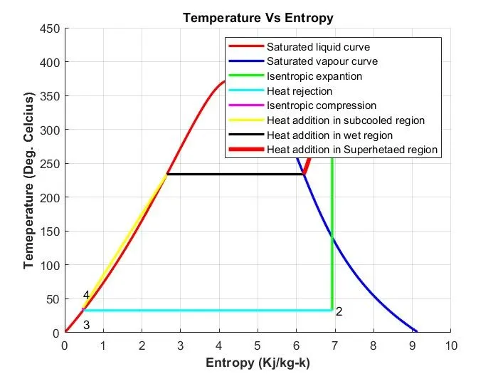
% Plotting T-S Diagram for Rankine Cycle
figure(1)
hold on
plot(sf,T,'color','b','linewidth',2,'color','r');
plot(sg,T,'color','b','linewidth',2,'color','b');
plot([s1 s2],[T1 T2], 'color', 'g','linewidth',2);
plot([s2 s3],[T2 T3], 'color', 'c', 'linewidth',2);
plot([s3 s4],[T3 T4], 'color', 'm', 'linewidth',2);
plot([s4 s5],[T4 T5], 'color', 'y', 'linewidth',2);
plot([s5 s6],[T5 T6], 'color', 'k', 'linewidth',2);

s_1 = linspace(s6,s1,1000);
for j = 1:length(s_1)
    Tc(j)= XSteam('T_ps',P1,s_1(j));
end

plot(s_1,Tc, 'color','r','linewidth',3.5)
legend('Saturated liquid curve','Saturated vapour curve','Isentropic expantion','Heat rejection','Isentropic compression','Heat addition in subcooled region','Heat addition in wet region','Heat addition in Superhetaed region')
grid on
text(s1+0.1, T1, '1')
text(s2+0.1, T2, '2')
text(s3, T3-20, '3')
text(s4, T4+20, '4')
title ('Temperature Vs Entropy','FontWeight','Bold')
xlabel ('Entropy (Kj/kg-k)', 'FontWeight','Bold')
ylabel ('Temeperature (Deg. Celcius)','FontWeight','Bold')

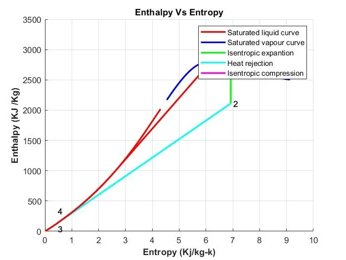
% Plotting H-S Diagram for Rankine Cycle
figure(2)
hold on
plot(sf,hf,'color','b','linewidth',2,'color','r');
plot(sg,hg ,'color','b','linewidth',2,'color','b');
plot ([s1 s2],[h1 h2],'color','g','linewidth' ,2);
plot ([s2 s3],[h2 h3],'color','c','linewidth' ,2);
plot ([s3 s4],[h3 h4],'color','m','linewidth',2);

hc = linspace(h4,h5,100);
for k = 1:length (hc)
         s_c(k) = XSteam ('s_ph' ,P1,hc (k));
end

plot(s_c ,hc ,'color','r ','linewidth',2)
plot ([s5 s6],[h5 h6],'color','r','linewidth',2)

for l = 1:length(s_1)
    h_c(l) = XSteam('h_ps',P1,s_1(l));
end

plot(s_1,h_c,'color','r','linewidth',3)
legend('Saturated liquid curve','Saturated vapour curve','Isentropic expantion','Heat rejection','Isentropic compression')
text(s1+0.1,h1,'1')
text(s2+0.1,h2,'2')
text(s3,h3-100,'3 ')
text(s4,h4+200,'4')
title('Enthalpy Vs Entropy','FontWeight','Bold')
xlabel('Entropy (Kj/kg-k)','FontWeight','Bold')
ylabel('Enthalpy (KJ /Kg)','FontWeight','Bold')
grid on


%  Displaying  Results  in  Command  window
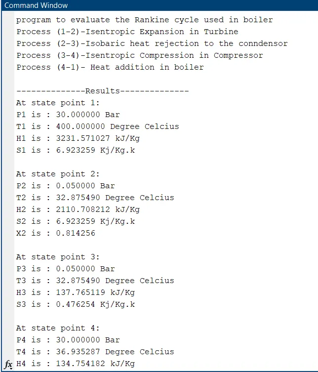
fprintf('\n--------------Results--------------\n')
fprintf('At state point 1:\n')
fprintf('P1 is : %f Bar\n',P1);
fprintf('T1 is : %f Degree Celcius\n',T1);
fprintf('H1 is : %f kJ/Kg\n',h1);
fprintf('S1 is : %f Kj/Kg.k\r\n',s1);

fprintf('At state point 2:\n')
fprintf('P2 is : %f Bar\n',P2);
fprintf('T2 is : %f Degree Celcius\n',T2);
fprintf('H2 is : %f kJ/Kg\n',h2);
fprintf('S2 is : %f Kj/Kg.k\n',s2);
fprintf('X2 is : %f \r\n',X2);

fprintf('At state point 3:\n')
fprintf('P3 is : %f Bar\n',P3);
fprintf('T3 is : %f Degree Celcius\n',T3);
fprintf('H3 is : %f kJ/Kg\n',h3);
fprintf('S3 is : %f Kj/Kg.k\r\n',s3);

fprintf('At state point 4:\n')
fprintf('P4 is : %f Bar\n',P4);
fprintf('T4 is : %f Degree Celcius\n',T4);
fprintf('H4 is : %f kJ/Kg\n',h4);
fprintf('S4 is : %f Kj/Kg.k\r\n',s4);

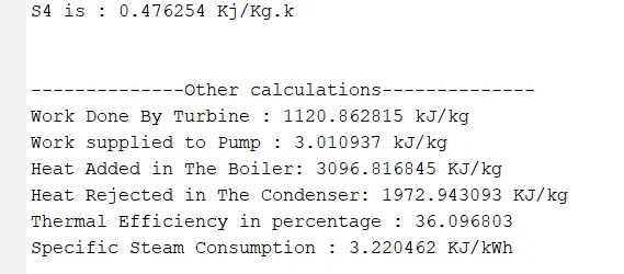
% Other calculations
fprintf('\n--------------Other calculations--------------\n')
fprintf ('Work Done By Turbine : %f kJ/kg\n',Wt)
fprintf ('Work supplied to Pump : %f kJ/kg\n',wp)
fprintf ('Heat Added in The Boiler: %f KJ/kg\n' ,Qin)
fprintf ('Heat Rejected in The Condenser: %f KJ/kg\n' ,Qout)
fprintf ('Thermal Efficiency in percentage : %f \n',Thermal_effi)
fprintf ('Specific Steam Consumption : %f KJ/kWh\r\n' ,SSC)
%%Output