Week 4.1 - Genetic Algorithm

AIM: To write a code in MATLAB to optimise the stalagmite function and find the global maxima of the function an plot the graphs.

OBJECTIVE:

• To study about the optimization process and to find out the optimum value.
• Study th statistical behaviour of unbounded, bounded and increase the no of iterations to find the global maxima
• Plot the graph for finding global maxima.

THEORY:

Optimization: Optimization is a decision making process it helps to find the best results under a set of prioritized criteria and constraints.It is a procedure which is executed iteratively by comparing various solutions is found.

Optimization refers to find a best values.

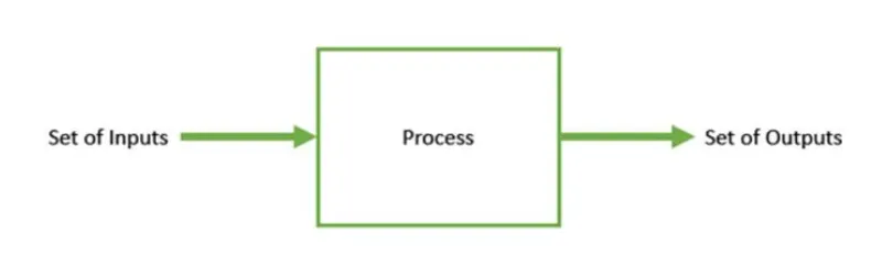
Example: While we are doing a problem , the steps and souces that we needed to take.

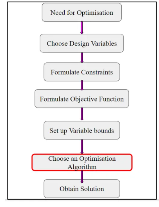
Stalagmite function:

1) A stalagmite function generally refers to the function with which we are generating values over a stalagmite kind of surface for finding out the local and global maxima and minima of that particular given function.

2)A stalagmite is an upward-growing mound of mineral deposits that have precipitated from water dripping onto the floor of a cave. Most stalagmites have rounded or flattened tips.

3)For this in Matlab we are using a method called 'Optimization'. It is a programming which does a selection of the best element with regard to some criterion from some set of population.

4) Optimization is done by systematically choosing input values ​​from within an allowed set and computing the results of the function.

5) In matlab to perform optimization we use 'Genetic Algorithm 'method which is a inbuild function in matlab to find the global maxima of that given stalagmite function.

Genetic Algorithm:

• Genetic algorithms (or GAs) are search and optimization techniques used in computing to find true or approximate solutions to specific problems.
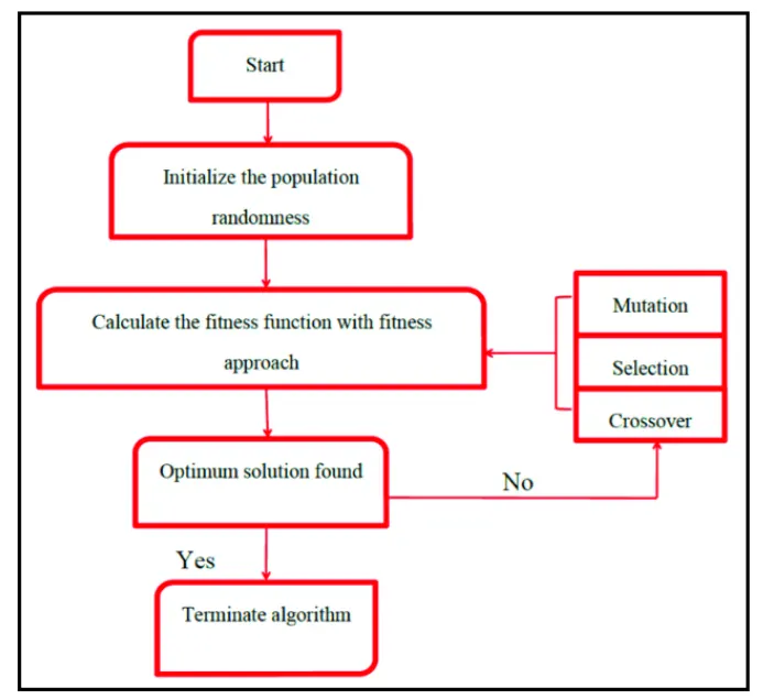
• Genetic algorithms are a particular class of evolutionary algorithms that use techniques inspired by evolutionary biology such as inheritance, mutation, selection, and crossover (also called recombination).
• These algorithms are based on Darwin’s principle of “Natural Selection” and “Genetic Inheritance”(Darwin1859)
  “Select The Best, Discard The Rest”
• GAs search a population of points in parallel, not a single point.
• GAs do not require derivative information or other auxiliary knowledge, only the objective function and corresponding fitness levels influence the directions of search. For this reason, GAs are often called blind search methods.
• GAs use probabilistic transition rules, not deterministic ones. This makes them more robust and applicable to a large range of problems.
• GAs work on an encoding of the parameters set rather than the parameters set itself.

The three techniques are:

Selection: A number of individuals is selected from the population in the mating pool. Based on the previously calculated fitness value, the best individuals based on a threshold are selected. After that step, we will end selecting a subset of the population in the mating pool.

Crossover: Crossover in GA generates new generation the same as natural mutation. By mutating the old generation parents, the new generation offspring comes by carrying genes from both parents. The amount of genes carried from each parent is random.

Mutation: For each offspring, select some genes and change its value. Mutation prevents the solution from falling into a local minima.

Fitness function:

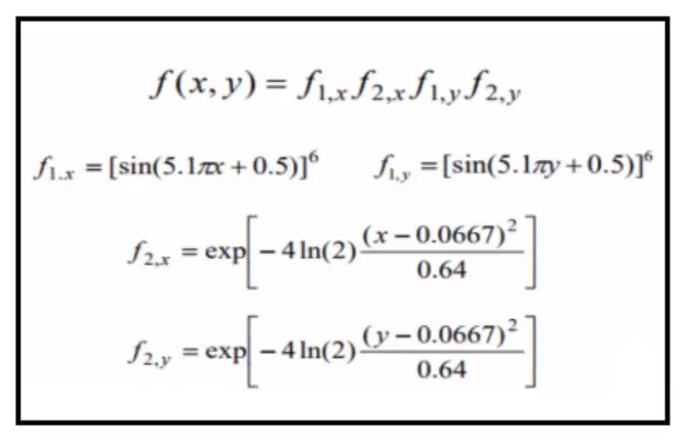
The formula we have used in function to find the minimum value, later we are going to multiply to find global maxima.

Syntax for genetic algorithm:

we can give the inputs by any one of the following ways-

x = ga(fun,nvars)

x = ga(fun,nvars,A,b)

x = ga(fun,nvars,A,b,Aeq,beq)

x = ga(fun,nvars,A,b,Aeq,beq,lb,ub)

x = ga(fun,nvars,A,b,Aeq,beq,lb,ub,nonlcon)

x = ga(fun,nvars,A,b,Aeq,beq,lb,ub,nonlcon,options)

x = ga(fun,nvars,A,b,[],[],lb,ub,nonlcon,IntCon)

x = ga(fun,nvars,A,b,[],[],lb,ub,nonlcon,IntCon,options)

x = ga(problem)

[x,fval] = ga(___)

[x,fval,exitflag,output] = ga(___)

[x,fval,exitflag,output,population,scores] = ga(___)

Description of input variables:

These are the various input syntaxes that can be given-

x = ga(fun,nvars) finds a local unconstrained minimum, x, to the objective function, fun. nvars is the dimension (number of design variables) of fun.

x = ga(fun,nvars,A,b) finds a local minimum x to fun, subject to the linear inequalities A*x ≤ b. ga evaluates the matrix product A*x as if x is transposed (A*x').

x = ga(fun,nvars,A,b,Aeq,beq) finds a local minimum x to fun, subject to the linear equalities Aeq*x = beq and A*x ≤ b. (Set A=[] and b=[] if no linear inequalities
exist.) ga evaluates the matrix product Aeq*x as if x is transposed (Aeq*x').

x = ga(fun,nvars,A,b,Aeq,beq,lb,ub) defines a set of lower and upper bounds on the design variables, x, so that a solution is found in the range lb ≤ x ≤ ub. (Set Aeq=[] and beq=[] if no linear equalities exist.)

x = ga(fun,nvars,A,b,Aeq,beq,lb,ub,nonlcon) subjects the minimization to the constraints defined in nonlcon. The function nonlcon accepts x and returns vectors C and Ceq,
representing the nonlinear inequalities and equalities respectively. ga minimizes the fun such that C(x) ≤ 0 and Ceq(x) = 0. (Set lb=[] and ub=[] if no bounds exist.)

x = ga(fun,nvars,A,b,Aeq,beq,lb,ub,nonlcon,options) minimizes with the default optimization parameters replaced by values in options. (Set nonlcon=[] if no nonlinear constraints exist.) Create options using optimoptions.

x = ga(fun,nvars,A,b,[],[],lb,ub,nonlcon,IntCon) or x = ga(fun,nvars,A,b,[],[],lb,ub,nonlcon,IntCon,options) requires that the variables listed in IntCon take integer values.
When there are integer constraints, ga does not accept linear or nonlinear equality constraints, only inequality constraints.

x = ga(problem) finds the minimum for problem, where problem is a structure.

Outputs from the functions:

[x,fval] = ga(___), for any previous input arguments, also returns fval, the value of the fitness function at x.

[x,fval,exitflag,output] = ga(___) also returns exitflag, an integer identifying the reason the algorithm terminated, and output, a structure that contains output from each generation and other information about the performance of the algorithm.

[x,fval,exitflag,output,population,scores] = ga(___) also returns a matrix population, whose rows are the final population, and a vector scores, the scores of the final population.

CODE:

The code for optimization and to find global maxima

clear all
close all
clc

% Inputs
x = linspace(0,0.6,150);
y = linspace(0,0.6,150);

% No of iterations
num_cases = 50

[xx yy] = meshgrid(x,y);

%Calling stalagmite function

for i = 1 : length(xx)
    for j = 1: length(yy)
        input_vector(1) = xx(i,j);
        input_vector(2) = yy(i,j);
        f(i,j) = stalagmite(input_vector);
    end
end

%study 1 Statistical behaviour with unbounded inputs

tic
for a = 1 : num_cases
    [input1,fopt1(a)] = ga(@stalagmite,2);
    xopt1(a) = input1(1);
    yopt1(a) = input1(2);
end
study_time = toc

figure(1)
subplot(2,1,1)
hold on
surfc(x,y,-f)
shading interp
plot3(xopt1,yopt1,-fopt1,'marker','o','markersize',5,'markerfacecolor','r')
title('Statistical behaviour with unbounded inputs')
subplot(2,1,2)
plot(-fopt1)
xlabel('iterations')
ylabel('function maxima')

%study2 statastical behaviour with bounded inputs
tic
for b = 1:num_cases
    [input2,fopt2(b)] = ga(@stalagmite,2,[],[],[],[],[0;0],[0.6;0.6]);
    xopt2(b) = input2(1);
    yopt2(b) = input2(2);
end
study_time1 = toc

figure(2)
subplot(2,1,1)
hold on
surfc(x,y,-f)
shading interp
plot3(xopt2,yopt2,-fopt2,'marker','o','markersize',5,'markerfacecolor','r')
title('statastical behaviour with bounded inputs')
subplot(2,1,2)
plot(-fopt2)
xlabel('iterations')
ylabel('function maxima')

%study3 Increasing ga iterations 

options = optimoptions('ga')
options = optimoptions(options,'populationsize',200);

tic
for c = 1:num_cases
    [input3,fopt3(c)] = ga(@stalagmite,2,[],[],[],[],[0;0],[1;1],[],[],options);
    xopt3(c) = input3(1);
    yopt3(c) = input3(2);
end
study2_time = toc


figure(3)
subplot(2,1,1)
hold on
surfc(x,y,-f)
shading interp
plot3(xopt3,yopt3,-fopt3,'marker','o','markersize',5,'markerfacecolor','r')
title('Increasing ga iterations')
subplot(2,1,2)
plot(-fopt3)
xlabel('iterations')
ylabel('function maxima')
    

The code for function optimization

function[f] = stalagmite(input_vector)
f1_x = (sin((5.1*pi*input_vector(1)) + 0.5))^6;
f1_y = (sin((5.1*pi*input_vector(2)) + 0.5))^6;
f2_x = exp((-4*log(2)*(input_vector(1)-0.0667)^2)/0.64);
f2_y = exp((-4*log(2)*(input_vector(2)-0.0667)^2)/0.64);
f = -(f1_x * f1_y * f2_x * f2_y);
end

Explanation:

• First we have give the linspace commands to the x and y arrays
• And number of iterations is to be 50 ( we can give as per our need)
• By using meshgrid command we define a plot for x and y arrays
• We have a written a function program to calculate the values of minimum value.
• By using the for loop, we call the function to this loop and calculated the minimum value.
• We have done a three studys here

Study1: Stattical behaviour with un bounded inputs - calculating the global maxima using the stalagmite optimization with statistical behaviour by creating a for loop and finding out the optimum values, also calculate time taken to complete the operation.Plot the stalagmite and optimum value in a subplot and foptimum values separately.

Study2: Statastical behaviour with bounded inputs - By calculating like above, the difference is change in syntax of ga. Upper and lower boundaries are used. Plot the graphs as mentioned above.

Study3: Increasing ga iterations - By calculating like above, the difference is change in syntax and by assinging the range of iterations.Plot the graphs as mentioned above.

RESULTS

1) Study 1 : Graph

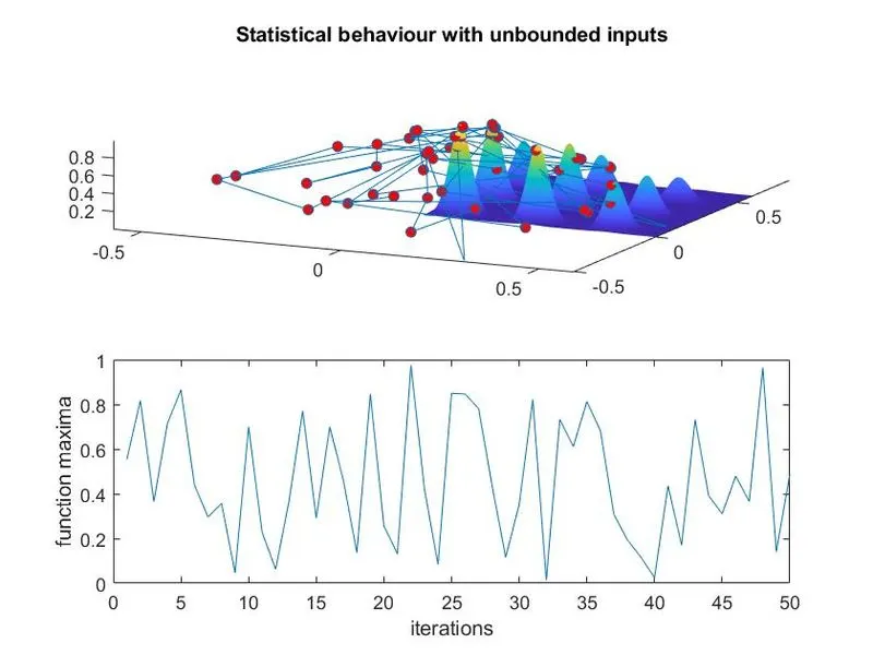
Study 1 : Study time: 3.2875 sec

2) Study 2 : Graph

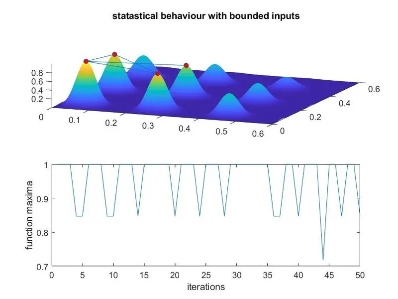
Study 2 : Study time: 4.1862 sec

3) Study 3 : Graph

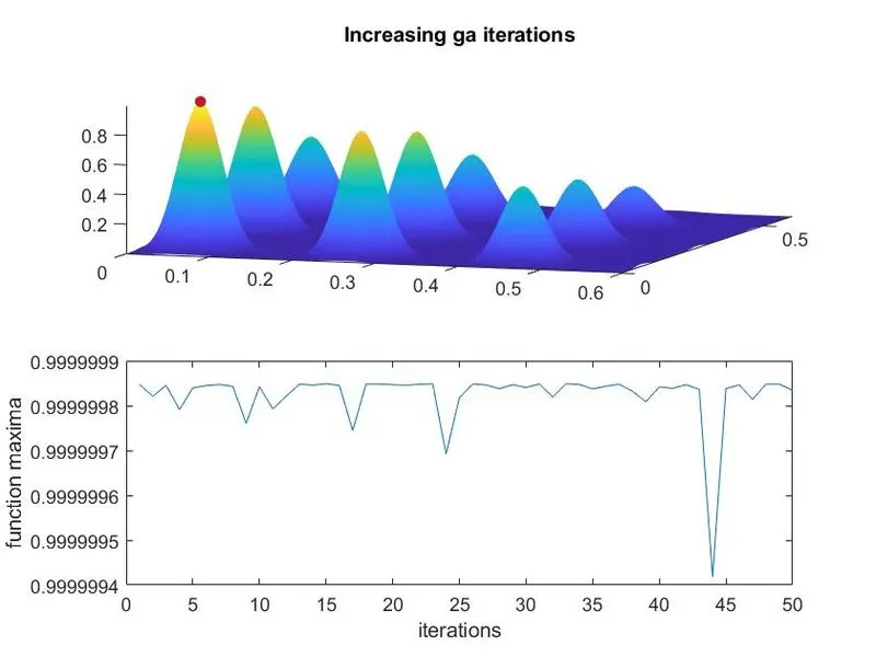
Study 3 : Study time: 10.0612 sec

CONCLUSION:

• To create a stagalmite function and find the optimum value by using matlab and plotted the curves.
• Learning the concept of geometric algorithm to find a global maxima.
• From the graphs we can say that 1st graph is Statstical behaviour of unbounded inputs, we get many minimum values. And the second graph is h is Statstical behaviour of bounded inputs within a limit. And 3rd graph is ga iterations,we got a global maxima.