Week 3 - Solving second order ODEs

AIM: To write a program that solves the ODE which represents the equation of a simple pendulum with damping.

OBJECTIVE: To create a animatiion of motion of simple pendulum by solving the ODE(ordinary differential equation) using matlab.

THEORY:

ODE is extremely important in engineering, they describe a lot of phenomena and helps to understands the system. One of the example is

Simple Pendulum:

• The motion of the simple pendulum describes the spring, mass and damper system
• We have an example like suspension system can be modeled like combination of spring, mass and damper.
• The 2nd order ODE for the simple pendulum with damping is

Here is the image of 2nd order ODE

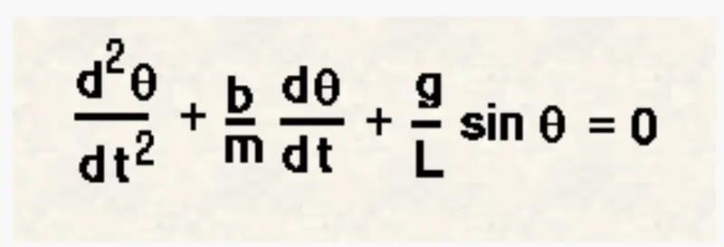
In the above equation,

g = gravity in m/s2,

L = length of the pendulum in m,

m = mass of the ball in kg,

b =damping coefficient.

• We will calulate (theta) and rate at which (theta) is changing w.r.t time(angular velocity)

Here we are assuming the values are

L=1 metre,

m=1 kg,

b=0.05.

g=9.81 m/s2.

angular velocity = 3 rad/sec

CODE:

Now we will write the code

clear all
close all
clc

% Inputs
b = 0.01;
g = 9.81;
l = 1;
m =0.1;

% Initial condition [There are two 1st order ODE's one for velocity and another for displacement)
theta_0 = [0;3];

% We are going to integrating the systemto obtain solution,for those we
% need to define a value for time
t_span = linspace(0,20,200);

% We have to call system ODE
[t,results] = ode45(@(t,theta) ode_func(t,theta,b,g,l,m),t_span,theta_0);

%Assume
 c = [t,results]
 ang = c(:,2)
 
 ct = 1;
 
 for i = 1:length(ang)
     x0 = 0
     y0 = 0
     
     x1 = -l * sind(ang(i))
     y1 = -l * cosd(ang(i))
     
    plot([x0 x1],[y0 y1],'linewidth',4)
    hold on
    % Use marker command to create sphere 
    plot(x0,y0,'marker','o','markersize',20,'markerfacecolor','r')
    plot(x1,y1,'marker','o','markersize',40,'markerfacecolor','g')
    
    axis([-0.03 0.02 -1.4 0.5])
    xlabel('x-displacement')
    ylabel('y-displacement')
    hold off
    pause(0.02)
    M(ct) = getframe(gcf)
    ct = ct+1;
 end
% For simulation
movie(M)
videofile = VideoWriter('Pendulum.avi','Uncompressed AVI')
open(videofile)
writeVideo(videofile,M)
close(videofile)

The fundemental idea behind solving ODE is, when we have higher order ODE then break down into 1st order ODE'S. For this we have written a function code that helps in main code:

function[dtheta_dt] = ode_func(t,theta,b,g,l,m)
             theta1 = theta(1);
             theta2 = theta(2);
         dtheta1_dt = theta2;
         dtheta2_dt = -(b/m)*theta2 - (g/l)*sin(theta1);
          dtheta_dt = [dtheta1_dt;dtheta2_dt];
end

• This is the breaking down of 2nd order ODE in to 1st order ODE

CODE LOGIC:

Here we have taken the coordinates like

• At the starting point , the pendulum one end is fixed. so the points are taken as

(x0,y0) = (0,0)

• Actually the line subjected to angle theta w.r.t X-axis is L * cos(theta) and similarly w.r.t Y-axis is L*sin(theta)
• But in this case, we are taken the angle theta w.r.t Y-axis, so the values become reverse.
• Now the coordinates are

x1 = -l * sind(ang(i))

x2 = -l * cosd(ang(i))

• And we are taken the values below the axis, so it should be negative.
• By insering the plot command we can assume it.

ode45: ODE45 is a function in matlab that solves ordinary or partial differential equations using a numerical method.

Syntax of ODE45:

[t,results] = ode45(@(x)x^2,tspan,y0)

For LOOP:

• The purpose of 'for' loop is to make number of iterations. so that it will take all the values of theta.
• We have number of values of theta, so it is difficult to create every value, so we inserted for loop command , so that it makes easy.
• In this 'for' loop works as it takes up to the length of angle, and gives the values of x1,y1 at each angle and generate output.
• We used VideoWriter command for animation

OUTPUTS:

Here is the link for the animation of simple pendulum

https://drive.google.com/file/d/1pUegcKhDZYEJ_dZIsTCqhzznY9tnQtYy/view?usp=sharing

• This shows how pendulum oscillates from one position to other position with a damping frequency
• For creating Sphere we used the 'marker' command, by giving color, shape,size.

CONCLUSION:

Finally i want to conclude that,

i) Program has been written that represents the equation of motion of a simple pendulum with damping.

ii) Created a animation of motion of simple pendulum by solving the ODE using Matlab.